ai
Introduction to ML
Machine learning is a field of inquiry devoted to understanding and building methods that 'learn', that is, methods that leverage data to improve performance on some set of tasks. It is seen as a part of artificial intelligence.
Key ML Terminology
Framing
What is (supervised) machine learning? Concisely put, it is the following:
- ML systems learn how to combine input to produce useful predictions on never-before-seen data.
Let's explore fundamental machine learning terminology.
Labels
A label is the thing we are predicting - the y variable in simple linear regression. The label could be the future price of wheat, the kind of animal shown in the picture, the meaning of an audio clip, or just about anything.
Features
A feature is an input variable - the x variable in simple linera regression. A simple machine learning project might use a single feature, while a more sophisticated machine learning project could use millions of features, specified as:
$$x1,x2,...,xn$$
In the "spam detector" example, the features could include the following:
- words in the email text
- sender's address
- time of day the email was sent
- email contains the phrase "one weird trick."
Examples
An example is a particular instance of data, x. (We put x in boldface to indicate that it is a vector.) We break examples into two categories:
- labeled examples
- unlabeled examples
A labeled example includes both feature(s) and the label. That is:
labeled examples: {features, label}: (x, y)
Use labeled examples to train the model. In our "span detector" example, the labeled examples would be individual emails that users have explicitly marked as "spam" or "not spam."
For example, the following table shows 5 labeled examples from a data set containing information about housing prices in California:
| HousingMedianAge (feature) | TotalRooms (feature) | TotalBedrooms (feature) | MedianHouseValue (feature) |
|---|---|---|---|
| 15 | 5612 | 1283 | 66900 |
| 19 | 7650 | 1901 | 80100 |
| 17 | 720 | 174 | 85700 |
| 14 | 1501 | 337 | 73400 |
| 20 | 1454 | 326 | 65500 |
An unlabeled example contains feature(s) but not the label. That is:
unlabeled examples: {features, ?}: (x, ?)
Here are 3 unlabeled examples from the same housing dataset, which exclude MedianHouseValue:
| HousingMedianAge (feature) | TotalRooms (feature) | TotalBedrooms (feature) |
|---|---|---|
| 42 | 1686 | 361 |
| 34 | 1226 | 180 |
| 33 | 1077 | 271 |
Once we've trained our model with labeled examples, we use that model to predict the label on unlabeled examples. In the spam detector, unlabeled examples are new emails that humans haven't yet labeled.
Models
A model defines the relationship between feature(s) and label. For example, a span detector might associate certain features strongly with "spam". Let's highlight two phases of a model's life:
Training means creating or learning the model. That is, you show the model labeled examples and enable the model to gradually learn the relationships between features and label.
Inference means applying the trained model to unlabeled examples. That is, you use the trained model to make useful predictions (
y'). For example, during inference, you can predict MedianHouseValue for new unlabeled examples.
Regression vs. classification
A regression model predicts continuous values. For example, regression models make predictions that answer questions like the following:
- What is the value of a house in California?
- What is the probability that a user will click on this ad?
A classification model predicts discrete values. For example, classification models make predictions that answer questions like the following:
- Is a given email message spam or not spam?
- Is this an image of a dog, a cat, or a hamster?
Descending into ML
Linear regression is a method for finding the straight line or hyperplane that best fits a set of points.
Linear Regression
It has long been known that crickets (an insect species) chirp more frequently on hotter days than on cooler days. For decades, professional and amateur scientists have cataloged data on chirps-per-minute and temperature. As a birthday gift, your Aunt Ruth gives you her cricket database and asks you to learn a model to predict this relationship. Using this data, you want to explore this relationship.
First, examine your data by plotting it:

Figure 1. Chirps per Minute vs. Temperature in Celsius.
As expected, the plot shows the temperature rising with the number of chirps. Is this relationship between chirps and temperature linear? Yes, you could draw a single straight line like the following to approximate this relationship:

Figure 2. A linear relationship.
True, the line doesn't pass through every dot, but the line does clearly show the relationship between chirps and temperature. Using the equation for a line, you could write down this relationship as follows:
$$y=mx+b$$
where:
- $y$ is the temperature in Celsius — the value we're trying to predict.
- $m$ is the slope of the line.
- $x$ is the number of chirps per minute — the value of our input feature.
- $b$ is the y-intercept.
By convention in machine learning, you'll write the equation for a model slightly differently:
$$y^\prime=b+w_{1}x_{1}$$
where:
- $y^\prime$ is a predicted label (a desired output).
- $b$ is the bias (the y-intercept), sometimes referred to as $w_{0}$.
- $w_{1}$ is the weight of feature 1. Weight is the same concept as the "slope" $m$ in the traditional equation of a line.
- $x_{1}$ is a feature (a known input).
To infer (predict) the temprature $y^\prime$ for new chirps-per-minute value $x_{1}$, just substitute the $x_{1}$ value into this model.
Although this model uses only one feature, a more sophisticated model might rely on multiple features, each having a separate weight ($w_{1}$, $w_{2}$, etc.). For example, a model that relies on three features might look as follows:
$$y^\prime=b+w_{1}x_{1}+w_{2}x_{2}+w_{3}x_{3}$$
Training and Loss
Training a model simply means learning (determining) good values for all the weights and the bias from labeled examples. In supervised learning, a machine learning algorithm builds a model by examining many examples and attempting to find a model that minimizes loss; this process is called empirical risk minimization.
Loss is the penalty for a bad prediction. That is, loss is a number indicating how bad the model's prediction was on a single example. If the model's prediction is perfect, the loss is zero; otherwise, the loss is greater. The goal of training a model is to find a set of weights and biases that have low loss, on average, across all examples. For example, Figure 3 shows a high loss model on the left and a low loss model on the right. Note the following about the figure:
- The arrows represent loss.
- The blue lines represent predictions.
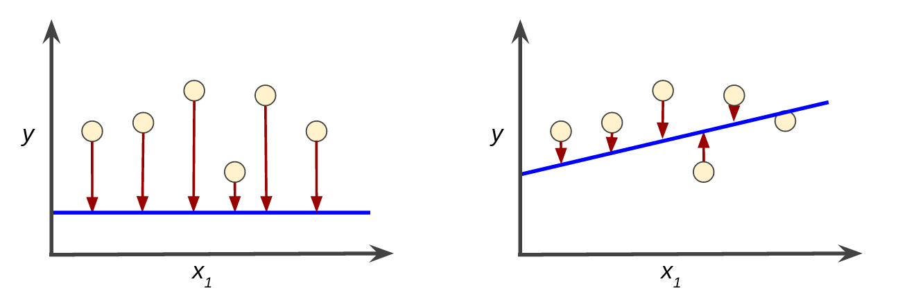
Figure 3. High loss in the left model; low loss in the right model.
Notice that the arrows in the left plot are much longer than their counterparts in the right plot. Clearly, the line in the right plot is a much better predictive model than the line in the left plot.
You might be wondering whether you could create a mathematical function — a loss function — that would aggregate the individual losses in a meaningful fashion.
Squared loss: a popular loss function
The linear regression models we'll examine here use a loss function called squared loss (also known as L2 loss). The squared loss for a single example is as follows:
  = the square of the difference between the label and the prediction
  = (observation - prediction(x))2
  = (y - y')2
Mean square error (MSE) is the average squared loss per example over the whole dataset. To calculate MSE, sum up all the squared losses for individual examples and then divide by the number of examples:
where:
- $(x,y)$ is an example in which
- $x$ is a set of features (for example chirps/minute, age, gender) that the model uses to make predictions.
- $y$ is the example's label (for example, temprature).
- $prediction(x)$ is a function of the weights and bias in combination with the sets of features $x$.
- $D$ is a dataset containing many labeled examples, which are $(x,y)$ pairs.
- $N$ is the number of examples in $D$.
Although MSE is commonly-used in machine learning, it is neither the only practical loss function nor the best loss function for all circumstances.
Reducing Loss
To train a model, we need a good way to reduce the model’s loss. An iterative approach is one widely used method for reducing loss, and is as easy and efficient as walking down a hill.
An iterative approach
Iterative learning might remind you of the "Hot and Cold" kid's game for finding a hidden object like a thimble. In this game, the "hidden object" is the best possible model. You'll start with a wild guess ("The value of $w_{1}$ is $0$.") and wait for the system to tell you what the loss is. Then, you'll try another guess ("The value of $w_{1}$ is $0.5$.") and see what the loss is. Aah, you're getting warmer. Actually, if you play this game right, you'll usually be getting warmer. The real trick to the game is trying to find the best possible model as efficiently as possible.
The following figure suggests the iterative trial-and-error process that machine learning algorithms use to train a model:

Figure 1. An iterative approach to training a model.
Iterative strategies are prevalent in machine learning, primarily because they scale so well to large data sets.
The "model" takes one or more features as input and returns one prediction ($y′$) as output. To simplify, consider a model that takes one feature and returns one prediction:
$$y′=b+w_{1}x_{1}$$
What initial values should we set for $b$ and $w_{1}$? For linear regression problems, it turns out that the starting values aren't important. We could pick random values, but we'll just take the following trivial values instead:
- $b=0$
- $w_{1}=0$
Suppose that the first feature value is 10. Plugging that feature value into the prediction function yields:
$$y′=0+0⋅10=0$$
The "Compute Loss" part of the diagram is the loss function that the model will use. Suppose we use the squared loss function. The loss function takes in two input values:
- $y′$: The model's prediction for features $x$
- $y$: The correct label corresponding to features $x$
At last, we've reached the "Compute parameter updates" part of the diagram. It is here that the machine learning system examines the value of the loss function and generates new values for $b$ and $w_{1}$. For now, just assume that this mysterious box devises new values and then the machine learning system re-evaluates all those features against all those labels, yielding a new value for the loss function, which yields new parameter values. And the learning continues iterating until the algorithm discovers the model parameters with the lowest possible loss. Usually, you iterate until overall loss stops changing or at least changes extremely slowly. When that happens, we say that the model has converged.
Gradient Descent
The iterative approach diagram contained a green hand-wavy box entitled "Compute parameter updates." We'll now replace that algorithmic fairy dust with something more substantial.
Suppose we had the time and the computing resources to calculate the loss for all possible values of $w_{1}$. For the kind of regression problems we've been examining, the resulting plot of loss vs. $w_{1}$ will always be convex. In other words, the plot will always be bowl-shaped, kind of like this:

Figure 2. Regression problems yield convex loss vs. weight plots.
Convex problems have only one minimum; that is, only one place where the slope is exactly 0. That minimum is where the loss function converges.
Calculating the loss function for every conceivable value of $w_{1}$ over the entire data set would be an inefficient way of finding the convergence point. Let's examine a better mechanism—very popular in machine learning—called gradient descent.
The first stage in gradient descent is to pick a starting value (a starting point) for $w_{1}$. The starting point doesn't matter much; therefore, many algorithms simply set $w_{1}$ to $0$ or pick a random value. The following figure shows that we've picked a starting point slightly greater than $0$:

Figure 3. A starting point for gradient descent.
The gradient descent algorithm then calculates the gradient of the loss curve at the starting point. Here in this Figure, the gradient of the loss is equal to the derivative (slope) of the curve, and tells you which way is "warmer" or "colder." When there are multiple weights, the gradient is a vector of partial derivatives with respect to the weights.
Partial derivatives
A multivariable function is a function with more than one argument, such as:
$$f(x,y)=e^{2y}\mathrm{sin}(x)$$
The partial derivate $f$ with respect to $x$, denoted as follows:
$$\dfrac{∂f}{∂x}$$
is a derivative of $f$ considered as a function of $x$ alone. To find the following:
$$\dfrac{∂f}{∂x}$$
so must hold $y$ constant (so $f$ is now a function of one variable $x$), and take the regular derivative of $f$ with respect to $x$. For example, when $y$ is fixed at $1$, the preceding function becomes:
$$f(x)=e^{2}\mathrm{sin}(x)$$
This is just a function of one variable $x$, whose derivative is:
$$e^{2}\mathrm{cos}(x)$$
In general, thinking of $y$ as fixed, the partial derivative of $f$ with respect to $x$ is calculated as follows:
$$\dfrac{∂f}{∂x}(x,y)=e^{2y}\mathrm{sin}(x)$$
Similarly, if we hold $x$ fixed instead, the partial derivative of $f$ with respect to $y$ is:
$$\dfrac{∂f}{∂x}(x,y)=2e^{2y}\mathrm{sin}(x)$$
Intuitively, a partial derivative tells how much the function changes when you perturb one variable a bit. In the preceding example:
$$\dfrac{\partial f}{\partial x}(0,1)=e^2 \approx 7.4$$
So when you start at $(0,1)$, hold $y$ constant, and move $x$ a little, $f$ changes by about $7.4$ times the amount that you changed $x$.
In machine learning, partial derivatives are mostly used in conjunction with the gradient of a function.
Gradients
The gradient of a function, denoted as follows, is the vector of partial derivatives with respect to all of the independent variables:
$$∇f$$
For instance, if:
$$f(x,y)=e^{2y}\mathrm{sin}(x)$$
then:
Note the following:
- $∇f$ - Points in the direction of greatest increase of the function.
- $−∇f$ - Points in the direction of greatest decrease of the function.
The number of dimensions in a vector is equal to the number of variables in the formula for $f$; in other words, the vector falls within the domain space of the function. For instance, the graph of the following function $f(x,y)$:
when viewed in three dimensions with $z=f(x,y)$ looks like a valley with a minimum at $(2,0,4)$:

The gradient of $f(x,y)$ is a two-dimensional vector that tells you in which $(x,y)$ direction to move for the maximum increase in height. Thus, the negative of the gradient moves you in the direction of maximum decrease in height. In other words, the negative of the gradient vector points into the valley.
In machine learning, gradients are used in gradient descent. We often have a loss function of many variables that we are trying to minimize, and we try to do this by following the negative of the gradient of the function.
Okay, so comming back to our gradient descent. We've found that a gradient is a vector that has both of the following characterstics:
- A direction
- A magnitude
The gradient always points in the direction of steepest increase in the loss function. The gradient descent algorithm takes a step in the direction of the negative gradient in order to reduce loss as quickly as possible.

Figure 4. Gradient descent relies on negative gradients.
To determine the next point along the loss function curve, the gradient descent algorithm adds some fraction of the gradient's magnitude to the starting point as shown in the following figure:

Figure 5. A gradient step moves us to the next point on the loss curve.
The gradient descent then repeats this process, edging ever closer to the minimum.
Learning Rate
As noted, the gradient vector has both a direction and a magnitude. Gradient descent algorithms multiply the gradient by a scalar known as the learning rate (also sometimes called step size) to determine the next point. For example, if the gradient magnitude is $2.5$ and the learning rate is $0.01$, then the gradient descent algorithm will pick the next point $0.025$ away from the previous point.
Hyperparameters are the knobs that programmers tweak in machine learning algorithms. Most machine learning programmers spend a fair amount of time tuning the learning rate. If you pick a learning rate that is too small, learning will take too long:

Figure 6. Learning rate is too small.
Conversely, if you specify a learning rate that is too large, the next point will perpetually bounce haphazardly across the bottom of the well like a quantum mechanics experiment gone horribly wrong:

Figure 7. Learning rate is too large.
There's a Goldilocks learning rate for every regression problem. The Goldilocks value is related to how flat the loss function is. If you know the gradient of the loss function is small then you can safely try a larger learning rate, which compensates for the small gradient and results in a larger step size.

Figure 8. Learning rate is just right.
The ideal learning rate in one-dimension is $\dfrac{1}{f(x)″}$ (the inverse of the second derivative of $f(x)$ at $x$).
The ideal learning rate for $2$ or more dimensions is the inverse of the Hessian (matrix of second partial derivatives).
The story for general convex functions is more complex.
Stochastic Gradient Descent
Stochastic Gradient Descent (SGD) is an optimization algorithm used to find the minimum of a function. It is a type of gradient descent algorithm that is often used in machine learning and deep learning. It is called "stochastic" because it uses random samples of the data to estimate the gradient of the objective function, rather than using the entire dataset.
Here's how it works:
- The algorithm starts with an initial guess of the parameters.
- It then selects a random sample of the data and calculates the gradient of the objective function with respect to the parameters using that sample.
- The parameters are then updated in the direction opposite to the gradient.
- This process is repeated until the parameters converge to a minimum of the objective function.
One of the main advantage of stochastic gradient descent is that it is computationally efficient. Because it uses a random sample of the data at each step, it can be much faster than batch gradient descent, which uses the entire dataset to calculate the gradient. Additionally, because it uses random samples, it can "escape" from local minima and converge to a global minimum.
An example of an application of SGD is Linear Regression, where the objective function is the mean squared error and the parameters are the weights of the model. Another example is Logistic Regression, where the objective function is the cross-entropy loss and the parameters are the weights of the model.
It should be noted that the optimization speed of SGD can be affected by the choice of the learning rate and the shuffling of the data during each iteration. Also it is not guaranteed to find the global minimum because of the randomness but it can be useful in practice.
In summary, Stochastic Gradient Descent is an optimization algorithm that is efficient and can help to find the global minimum of a function. It has been widely used in machine learning and deep learning tasks.
Generalization
Generalization refers to your model's ability to adapt properly to new, previously unseen data, drawn from the same distribution as the one used to create the model.
Peril of Overfitting
This module focuses on generalization. In order to develop some intuition about this concept, you're going to look at three figures. Assume that each dot in these figures represents a tree's position in a forest. The two colors have the following meanings:
- The blue dots represent sick trees.
- The orange dots represent healthy trees.
With that in mind, take a look at Figure 1.
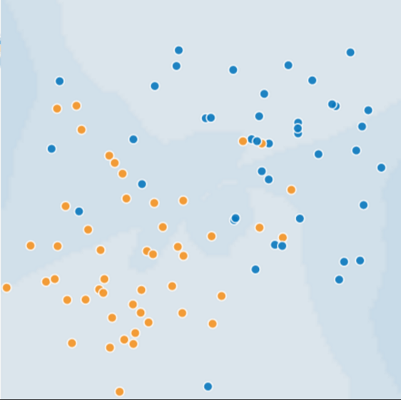
Figure 1. Sick (blue) and healthy (orange) trees.
Can you imagine a good model for predicting subsequent sick or healthy trees? Take a moment to mentally draw an arc that divides the blues from the oranges, or mentally lasso a batch of oranges or blues. Then, look at Figure 2, which shows how a certain machine learning model separated the sick trees from the healthy trees. Note that this model produced a very low loss.
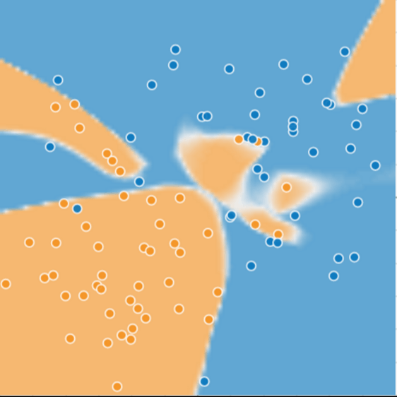
Figure 2. A complex model for distinguishing sick from healthy trees.
> At first glance, the model shown in Figure 2 appeared to do an excellent job of separating the healthy trees from the sick ones. Or did it?
Low loss, but still a bad model?
Figure 3 shows what happened when we added new data to the model. It turned out that the model adapted very poorly to the new data. Notice that the model miscategorized much of the new data.
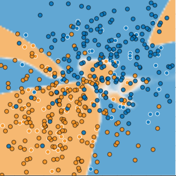
Figure 3. The model did a bad job predicting new data.
The model shown in Figures 2 and 3 overfits the peculiarities of the data it trained on. An overfit model gets a low loss during training but does a poor job predicting new data. If a model fits the current sample well, how can we trust that it will make good predictions on new data? As you'll see later on, overfitting is caused by making a model more complex than necessary. The fundamental tension of machine learning is between fitting our data well, but also fitting the data as simply as possible.
Machine learning's goal is to predict well on new data drawn from a (hidden) true probability distribution. Unfortunately, the model can't see the whole truth; the model can only sample from a training data set. If a model fits the current examples well, how can you trust the model will also make good predictions on never-before-seen examples?
William of Ockham, a 14th century friar and philosopher, loved simplicity. He believed that scientists should prefer simpler formulas or theories over more complex ones. To put Ockham's razor in machine learning terms:
> The less complex an ML model, the more likely that a good empirical result is not just due to the peculiarities of the sample.
In modern times, we've formalized Ockham's razor into the fields of statistical learning theory and computational learning theory. These fields have developed generalization bounds ̶ a statistical description of a model's ability to generalize to new data based on factors such as:
- the complexity of the model
- the model's performance on training data
A machine learning model aims to make good predictions on new, previously unseen data. But if you are building a model from your data set, how would you get the previously unseen data? Well, one way is to divide your data set into two subsets:
- training set — a subset to train a model.
- test set — a subset to test the model.
Good performance on the test set is a useful indicator of good performance on the new data in general, assuming that:
- The test set is large enough.
- You don't cheat by using the same test set over and over.
The ML fine print
The following three basic assumptions guide generalization:
- We draw examples independently and identically (i.i.d) at random from the distribution. In other words, examples don't influence each other. (An alternate explanation: i.i.d. is a way of referring to the randomness of variables.)
- The distribution is stationary; that is the distribution doesn't change within the data set.
- We draw examples from partitions from the same distribution.
In practice, we sometimes violate these assumptions. For example:
- Consider a model that chooses ads to display. The i.i.d. assumption would be violated if the model bases its choice of ads, in part, on what ads the user has previously seen.
- Consider a data set that contains retail sales information for a year. User's purchases change seasonally, which would violate stationarity.
When we know that any of the preceding three basic assumptions are violated, we must pay careful attention to metrics.
Training and Test Sets
A test set is a data set used to evaluate the model developed from a training set.
Splitting Data
- training set - a subset to train a model.
- test set - a subset to test the trained model.
You could imagine slicing the single data set as follows:

Figure 1. Slicing a single data set into a training set and test set.
Make sure that your test set meets the following two conditions:
- Is large enough to yield statistically meaningful results.
- Is representative of the data set as a whole. In other words, don't pick a test set with different characterstics than the training set.
Assuming that your test set meets the preceding two conditions, your goal is to create a model that generalizes well to new data. Our test set serves as a proxy for new data. For example, consider the following figure. Notice that the model learned for the training data is very simple. This model doesn't do a perfect job—a few predictions are wrong. However, this model does about as well on the test data as it does on the training data. In other words, this simple model does not overfit the training data.

Figure 2. Validating the trained model against test data.
Never train on test data. If you are seeing surprisingly good results on your evaluation metrics, it might be a sign that you are accidentally training on the test set. For example, high accuracy might indicate that test data has leaked into the training set.
For example, consider a model that predicts whether an email is spam, using the subject line, email body, and sender's email address as features. We apportion the data into training and test sets, with an 80-20 split. After training, the model achieves 99% precision on both the training set and the test set. We'd expect a lower precision on the test set, so we take another look at the data and discover that many of the examples in the test set are duplicates of examples in the training set (we neglected to scrub duplicate entries for the same spam email from our input database before splitting the data). We've inadvertently trained on some of our test data, and as a result, we're no longer accurately measuring how well our model generalizes to new data.
Validation Set
Partitioning a data set into a training set and test set lets you judge whether a given model will generalize well to new data. However, using only two partitions may be insufficient when doing many rounds of hyperparameter tuning.
Another Partition
Previously, we worked on two partitions of our data set and with those two partitions, the workflow could look as follows:

Figure 1. A possible workflow?
In the figure, "Tweak model" means adjusting anything about the model you can dream up—from changing the learning rate, to adding or removing features, to designing a completely new model from scratch. At the end of this workflow, you pick the model that does best on the test set.
Dividing the data set into two sets is a good idea, but not a panacea. You can greatly reduce your chances of overfitting by partitioning the data set into the three subsets shown in the following figure:

Figure 2. Slicing a single data set into three subsets.
Use the validation set to evaluate results from the training set. Then, use the test set to double-check your evaluation after the model has "passed" the validation set. The following figure shows this new workflow:

Figure 3. A better workflow.
In this improved workflow:
- Pick the model that does best on the validation set.
- Double-check that model against the test set.
This is a better workflow because it creates fewer exposures to the test set.
Representation
A machine learning model can't directly see, hear, or sense input examples. Instead, you must create a representation of the data to provide the model with a useful vantage point into the data's key qualities. That is, in order to train a model, you must choose the set of features that best represent the data.
Feature Engineering
In traditional programming, the focus is on code. In machine learning projects, the focus shifts to representation. That is, one way developers hone a model is by adding and improving its features.
Mapping Raw Data to Features
The left side of Figure 1 illustrates raw data from an input data source; the right side illustrates a feature vector, which is the set of floating-point values comprising the examples in your data set. Feature engineering means transforming raw data into a feature vector. Expect to spend significant time doing feature engineering.
Many machine learning models must represent the features as real-numbered vectors since the feature values must be multiplied by the model weights.

Figure 1. Feature engineering maps raw data to ML features.
Mapping numeric values
Integer and floating-point data don't need a special encoding because they can be multiplied by a numeric weight. As suggested in Figure 2, converting the raw integer value 6 to the feature value 6.0 is trivial:

Figure 2. Mapping integer values to floating-point values.
Mapping categorical values
Categorical features have a discrete set of possible values. For example, there might be a feature called street_name with options that include:
{'Charleston Road', 'North Shoreline Boulevard', 'Shorebird Way', 'Rengstorff Avenue'}
Since models cannot multiply strings by the learned weights, we use feature engineering to convert strings to numeric values.
We can accomplish this by defining a mapping from the feature values, which we'll refer to as the vocabulary of possible values, to integers. Since not every street in the world will appear in our dataset, we can group all other streets into a catch-all "other" category, known as an OOV (out-of-vocabulary) bucket.
Using this approach, here's how we can map our street names to numbers:
- map Charleston Road to 0
- map North Shoreline Boulevard to 1
- map Shorebird Way to 2
- map Rengstorff Avenue to 3
- map everything else (OOV) to 4
However, if we incorporate these index numbers directly into our model, it will impose some constraints that might be problematic:
- We'll be learning a single weight that applies to all streets. For example, if we learn a weight of 6 for
street_name, then we will multiply it by 0 for Charleston Road, by 1 for North Shoreline Boulevard, 2 for Shorebird Way and so on. Consider a model that predicts house prices usingstreet_nameas a feature. It is unlikely that there is a linear adjustment of price based on the street name, and furthermore this would assume you have ordered the streets based on their average house price. Our model needs the flexibility of learning different weights for each street that will be added to the price estimated using the other features. - We aren't accounting for cases where
street_namemay take multiple values. For example, many houses are located at the corner of two streets, and there's no way to encode that information in thestreet_namevalue if it contains a single index.
To remove both these constraints, we can instead create a binary vector for each categorical feature in our model that represents values as follows:
- For values that apply to the example, set corresponding vector elements to
1. - Set all other elements to
0.
The length of this vector is equal to the number of elements in the vocabulary. This representation is called a one-hot encoding when a single value is 1, and a multi-hot encoding when multiple values are 1.
Figure 3 illustrates a one-hot encoding of a particular street: Shorebird Way. The element in the binary vector for Shorebird Way has a value of 1, while the elements for all other streets have values of 0.

Figure 3. Mapping street address via one-hot encoding.
This approach effectively creates a Boolean variable for every feature value (e.g., street name). Here, if a house is on Shorebird Way then the binary value is 1 only for Shorebird Way. Thus, the model uses only the weight for Shorebird Way.
Similarly, if a house is at the corner of two streets, then two binary values are set to 1, and the model uses both their respective weights.
Sparse Representation
Suppose that you had 1,000,000 different street names in your data set that you wanted to include as values for street_name. Explicitly creating a binary vector of 1,000,000 elements where only 1 or 2 elements are true is a very inefficient representation in terms of both storage and computation time when processing these vectors. In this situation, a common approach is to use a sparse representation in which only nonzero values are stored. In sparse representations, an independent model weight is still learned for each feature value, as described above.
Qualities of Good Features
We've explored ways to map raw data into suitable feature vectors, but that's only part of the work. We must now explore what kinds of values actually make good features within those feature vectors.
Avoid rarely used discrete feature values
Good feature values should appear more than 5 or so times in a data set. Doing so enables a model to learn how this feature value relates to the label. That is, having many examples with the same discrete value gives the model a chance to see the feature in different settings, and in turn, determine when it's a good predictor for the label. For example, a house_type feature would likely contain many examples in which its value was victorian:
house_type: 'victorian'
Conversely, if a feature's value appears only once or very rarely, the model can't make predictions based on that feature. For example, unique_house_id is a bad feature because each value would be used only once, so the model couldn't learn anything from it:
unique_house_id: '8SK982ZZ1242Z'
Prefer clear and obvious meanings
Each feature should have a clear and obvious meaning to anyone on the project. For example, the following good feature is clearly named and the value makes sense with respect to the name:
house_age_years: 27
Conversely, the meaning of the following feature value is pretty much indecipherable to anyone but the engineer who created it:
house_age: 851472000
In some cases, noisy data (rather than bad engineering choices) causes unclear values. For example, the following user_age_years came from a source that didn't check for appropriate values:
user_age_years: 277
Don't mix "magic" values with actual data
Good floating-point features don't contain peculiar out-of-range discontinuities or "magic" values. For example, suppose a feature holds a floating-point value between 0 and 1. So, values like the following are fine:
quality_rating: 0.82
quality_rating: 0.37
However, if a user didn't enter a quality_rating, perhaps the data set represented its absence with a magic value like the following:
quality_rating: -1
To explicitly mark magic values, create a Boolean feature that indicates whether or not a quality_rating was supplied. Give this Boolean feature a name like is_quality_rating_defined.
In the original feature, replace the magic values as follows:
- For variables that take a finite set of values (discrete variables), add a new value to the set and use it to signify that the feature value is missing.
- For continuous variables, ensure missing values do not affect the model by using the mean value of the feature's data.
Account for upstream instability
The definition of a feature shouldn't change over time. For example, the following value is useful because the city name probably won't change. (Note that we'll still need to convert a string like "br/sao_paulo" to a one-hot vector.)
city_id: 'br/sao_paulo'
But gathering a value inferred by another model carries additional costs. Perhaps the value "219" currently represents Sao Paulo, but that representation could easily change on a future run of the other model:
inferred_city_cluster: 219
Cleaning Data
Apple trees produce some mixture of great fruit and wormy messes. Yet the apples in high-end grocery stores display 100% perfect fruit. Between orchard and grocery, someone spends significant time removing the bad apples or throwing a little wax on the salvageable ones. As an ML engineer, you'll spend enormous amounts of your time tossing out bad examples and cleaning up the salvageable ones. Even a few "bad apples" can spoil a large data set.
Scaling feature values
Scaling means converting floating-point feature values from their natural range (for example, 100 to 900) into a standard range (for example, 0 to 1 or -1 to +1). If a feature set consists of only a single feature, then scaling provides little to no practical benefit. If, however, a feature set consists of multiple features, then feature scaling provides the following benefits:
- Helps gradient descent converge more quickly.
- Helps avoid the "NaN trap," in which one number in the model becomes a NaN (e.g., when a value exceeds the floating-point precision limit during training), and—due to math operations—every other number in the model also eventually becomes a NaN.
- Helps the model learn appropriate weights for each feature. Without feature scaling, the model will pay too much attention to the features having a wider range.
You don't have to give every floating-point feature exactly the same scale. Nothing terrible will happen if Feature A is scaled from -1 to +1 while Feature B is scaled from -3 to +3. However, your model will react poorly if Feature B is scaled from 5000 to 100000.
One obvious way to scale numerical data is to linearly map [min value, max value] to a small scale, such as [-1, +1].
Another popular scaling tactic is to calculate the Z score of each value. The Z score relates the number of standard deviations away from the mean. In other words:
For example, given:
- mean = 100
- standard deviation = 20
- original value = 130
then:
scaled_value = (130 - 100) / 20
scaled_value = 1.5
Scaling with Z scores means that most scaled values will be between -3 and +3, but a few values will be a little higher or lower than that range.
Handling extreme outliers
The following plot represents a feature called roomsPerPerson from the California Housing data set. The value of roomsPerPerson was calculated by dividing the total number of rooms for an area by the population for that area. The plot shows that the vast majority of areas in California have one or two rooms per person. But take a look along the x-axis.

Figure 4. A verrrrry lonnnnnnng tail.
How could we minimize the influence of those extreme outliers? Well, one way would be to take the log of every value:

Figure 5. Logarithmic scaling still leaves a tail.
Log scaling does a slightly better job, but there's still a significant tail of outlier values. Let's pick yet another approach. What if we simply "cap" or "clip" the maximum value of roomsPerPerson at an arbitrary value, say 4.0?

Figure 6. Clipping feature values at 4.0
Clipping the feature value at 4.0 doesn't mean that we ignore all values greater than 4.0. Rather, it means that all values that were greater than 4.0 now become 4.0. This explains the funny hill at 4.0. Despite that hill, the scaled feature set is now more useful than the original data.
Binning
The following plot shows the relative prevalence of houses at different latitudes in California. Notice the clustering — Los Angeles is about at latitude 34 and San Francisco is roughly at latitude 38.

Figure 7. Houses per latitude.
In the data set, latitude is a floating-point value. However, it doesn't make sense to represent latitude as a floating-point feature in our model. That's because no linear relationship exists between latitude and housing values. For example, houses in latitude 35 are not $\dfrac{35}{34}$ more expensive (or less expensive) than houses at latitude 34. And yet, individual latitudes probably are a pretty good predictor of house values.
To make latitude a helpful predictor, let's divide latitudes into "bins" as suggested by the following figure:

Figure 8. Binning values.
Instead of having one floating-point feature, we now have 11 distinct boolean features (LatitudeBin1, LatitudeBin2, ..., LatitudeBin11). Having 11 separate features is somewhat inelegant, so let's unite them into a single 11-element vector. Doing so will enable us to represent latitude 37.4 as follows:
[0, 0, 0, 0, 0, 1, 0, 0, 0, 0, 0]
Thanks to binning, our model can now learn completely different weights for each latitude.
For simplicity's sake in the latitude example, we used whole numbers as bin boundaries. Had we wanted finer-grain resolution, we could have split bin boundaries at, say, every tenth of a degree. Adding more bins enables the model to learn different behaviors from latitude 37.4 than latitude 37.5, but only if there are sufficient examples at each tenth of a latitude.
Another approach is to bin by quantile, which ensures that the number of examples in each bucket is equal. Binning by quantile completely removes the need to worry about outliers.
Scrubbing
Until now, we've assumed that all the data used for training and testing was trustworthy. In real-life, many examples in data sets are unreliable due to one or more of the following:
- Omitted values. For instance, a person forgot to enter a value for a house's age.
- Duplicate examples. For example, a server mistakenly uploaded the same logs twice.
- Bad labels. For instance, a person mislabeled a picture of an oak tree as a maple.
- Bad feature values. For example, someone typed in an extra digit, or a thermometer was left out in the sun.
Once detected, you typically "fix" bad examples by removing them from the data set. To detect omitted values or duplicated examples, you can write a simple program. Detecting bad feature values or labels can be far trickier.
In addition to detecting bad individual examples, you must also detect bad data in the aggregate. Histograms are a great mechanism for visualizing your data in the aggregate. In addition, getting statistics like the following can help:
- Maximum and minimum
- Mean and median
- Standard deviation
Consider generating lists of the most common values for discrete features. For example, do the number of examples with country:uk match the number you expect. Should language:jp really be the most common language in your data set?
Know your data
Follow these rules:
- Keep in mind what you think your data should look like.
- Verify that the data meets these expectations (or that you can explain why it doesn’t).
- Double-check that the training data agrees with other sources (for example, dashboards).
Treat your data with all the care that you would treat any mission-critical code. Good ML relies on good data.
Feature Crosses
A feature cross is a synthetic feature formed by multiplying (crossing) two or more features. Crossing combinations of features can provide predictive abilities beyond what those features can provide individually.
Encoding Nonlinearity
In Figures 1 and 2, imagine the following:
- The blue dots represent sick trees.
- The orange dots represent healthy trees.
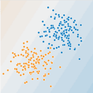
Figure 1. Is this a linear problem?
Can you draw a line that neatly separates the sick trees from the healthy trees? Sure. This is a linear problem. The line won't be perfect. A sick tree or two might be on the "healthy" side, but your line will be a good predictor.
Now look at the following figure:
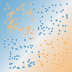
Figure 2. Is this a linear problem?
Can you draw a single straight line that neatly separates the sick trees from the healthy trees? No, you can't. This is a nonlinear problem. Any line you draw will be a poor predictor of tree health.
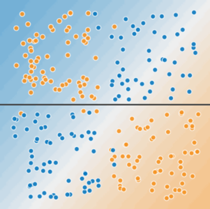
Figure 3. A single line can't separate the two classes.
To solve the nonlinear problem shown in Figure 2, create a feature cross. A feature cross is a synthetic feature that encodes nonlinearity in the feature space by multiplying two or more input features together. (The term cross comes from cross product.) Let's create a feature cross named $x_{3}$ by crossing $x_{1}$ and $x_{2}$:
$$x_{3}=x_{1}x_{2}$$
We treat this newly minted $x_{3}$ feature cross just like any other feature. The linear formula becomes:
A linear algorithm can learn a weight for $w_{3}$ just as it would for $w_{1}$ and $w_{2}$. In other words, although $w_{3}$ encodes nonlinear information, you don’t need to change how the linear model trains to determine the value of $w_{3}$.
Kinds of feature crosses
We can create many different kinds of feature crosses. For example:
[A X B]: a feature cross formed by multiplying the values of two features.[A x B x C x D x E]: a feature cross formed by multiplying the values of five features.[A x A]: a feature cross formed by squaring a single feature.
Thanks to stochastic gradient descent, linear models can be trained efficiently. Consequently, supplementing scaled linear models with feature crosses has traditionally been an efficient way to train on massive-scale data sets.
Crossing One-Hot Vectors
So far, we've focused on feature-crossing two individual floating-point features. In practice, machine learning models seldom cross continuous features. However, machine learning models do frequently cross one-hot feature vectors. Think of feature crosses of one-hot feature vectors as logical conjunctions. For example, suppose we have two features: country and language. A one-hot encoding of each generates vectors with binary features that can be interpreted as country=USA, country=France or language=English, language=Spanish. Then, if you do a feature cross of these one-hot encodings, you get binary features that can be interpreted as logical conjunctions, such as:
country: 'usa' AND language: 'spanish'
As another example, suppose you bin latitude and longitude, producing separate one-hot five-element feature vectors. For instance, a given latitude and longitude could be represented as follows:
binned_latitude = [0, 0, 0, 1, 0]
binned_longitude = [0, 1, 0, 0, 0]
Suppose you create a feature cross of these two feature vectors:
binned_latitude X binned_longitude
This feature cross is a 25-element one-hot vector (24 zeroes and 1 one). The single 1 in the cross identifies a particular conjunction of latitude and longitude. Your model can then learn particular associations about that conjunction.
Suppose we bin latitude and longitude much more coarsely, as follows:
binned_latitude(lat) = [
  0  < lat <= 10
  10 < lat <= 20
  20 < lat <= 30
]

binned_longitude(lon) = [
  0  < lon <= 15
  15 < lon <= 30
]
Creating a feature cross of those coarse bins leads to synthetic feature having the following meanings:
binned_latitude_X_longitude(lat, lon) = [
  0  < lat <= 10 AND 0  < lon <= 15
  0  < lat <= 10 AND 15 < lon <= 30
  10 < lat <= 20 AND 0  < lon <= 15
  10 < lat <= 20 AND 15 < lon <= 30
  20 < lat <= 30 AND 0  < lon <= 15
  20 < lat <= 30 AND 15 < lon <= 30
]
Now suppose our model needs to predict how satisfied dog owners will be with dogs based on two features:
- Behavior type (barking, crying, snuggling, etc.)
- Time of day
If we build a feature cross from both these features:
[behavior_type X time_of_day]
then we'll end up with vastly more predictive ability than either feature on its own. For example, if a dog cries (happily) at 5:00 pm when the owner returns from work will likely be a great positive predictor of owner satisfaction. Crying (miserably, perhaps) at 3:00 am when the owner was sleeping soundly will likely be a strong negative predictor of owner satisfaction.
Linear learners scale well to massive data. Using feature crosses on massive data sets is one efficient strategy for learning highly complex models. Neural networks provide another strategy.
Transform Your Data
Introduction to Transforming Data
Feature engineering is the process of determining which features might be useful in training a model, and then creating those features by transforming raw data found in log files and other sources. In this section, we focus on when and how to transform numeric and categorical data, and the tradeoffs of different approaches.
Reasons for Data Transformation
We transform features primarily for the following reasons:
Mandatory transformations for data compatibility. Examples include:
Converting non-numeric features into numeric. You can’t do matrix multiplication on a string, so we must convert the string to some numeric representation.
Resizing inputs to a fixed size. Linear models and feed-forward neural networks have a fixed number of input nodes, so your input data must always have the same size. For example, image models need to reshape the images in their dataset to a fixed size.
Optional quality transformations that may help the model perform better. Examples include:
Tokenization or lower-casing of text features.
Normalized numeric features (most models perform better afterwards).
Allowing linear models to introduce non-linearities into the feature space.
Where to Transform?
You can apply transformations either while generating the data on disk, or within the model.
Transforming prior to training
In this approach, we perform the transformation before training. This code lives separate from your machine learning model.
Pros
- Computation is performed only once.
- Computation can look at entire dataset to determine the transformation.
Cons
- Transformations need to be reproduced at prediction time. Beware of skew!
- Any transformation changes require rerunning data generation, leading to slower iterations.
Skew is more dangerous for cases involving online serving. In offline serving, you might be able to reuse the code that generates your training data. In online serving, the code that creates your dataset and the code used to handle live traffic are almost necessarily different, which makes it easy to introduce skew.
Transforming within the model
In this approach, the transformation is part of the model code. The model takes in untransformed data as input and will transform it within the model.
Pros
- Easy iterations. If you change the transformations, you can still use the same data files.
- You're guaranteed the same transformations at training and prediction time.
Cons
- Expensive transforms can increase model latency.
- Transformations are per batch.
There are many considerations for transforming per batch. Suppose you want to normalize a feature by its average value--that is, you want to change the feature values to have mean 0 and standard deviation 1. When transforming inside the model, this normalization will have access to only one batch of data, not the full dataset. You can either normalize by the average value within a batch (dangerous if batches are highly variant), or precompute the average and fix it as a constant in the model.
Explore, Clean, and Visualize Your Data
Explore and clean up your data before performing any transformations on it. You may have done some of the following tasks as you collected and constructed your dataset:
- Examine several rows of data.
- Check basic statistics.
- Fix missing numerical entries.
Visualize your data frequently. Graphs can help find anomalies or patterns that aren't clear from numerical statistics. Therefore, before getting too far into analysis, look at your data graphically, either via scatter plots or histograms. View graphs not only at the beginning of the pipeline, but also throughout transformation. Visualizations will help you continually check your assumptions and see the effects of any major changes.
Transforming Numeric Data
You may need to apply two kinds of transformations to numeric data:
- Normalizing - transforming numeric data to the same scale as other numeric data.
- Bucketing - transforming numeric (usually continuous) data to categorical data.
Why Normalize Numeric Features?
We strongly recommend normalizing a data set that has numeric features covering distinctly different ranges (for example, age and income). When different features have different ranges, gradient descent can "bounce" and slow down convergence. Optimizers like Adagrad and Adam protect against this problem by creating a separate effective learning rate for each feature.
We also recommend normalizing a single numeric feature that covers a wide range, such as "city population." If you don't normalize the "city population" feature, training the model might generate NaN errors. Unfortunately, optimizers like Adagrad and Adam can't prevent NaN errors when there is a wide range of values within a single feature.
Warning: When normalizing, ensure that the same normalizations are applied at serving time to avoid skew.
Normalization
The goal of normalization is to transform features to be on a similar scale. This improves the performance and training stability of the model.
Four common normalization techniques may be useful:
- scaling to a range
- clipping
- log scaling
- z-score
The following charts show the effect of each normalization technique on the distribution of the raw feature (price) on the left. The charts are based on the data set from 1985 Ward's Automotive Yearbook that is part of the UCI Machine Learning Repository under Automobile Data Set.

Figure 1. Summary of normalization techniques.
Scaling to a range
Recall from MLCC that scaling means converting floating-point feature values from their natural range (for example, 100 to 900) into a standard range—usually 0 and 1 (or sometimes -1 to +1). Use the following simple formula to scale to a range:
$$x' = \dfrac{(x - x_{min})}{(x_{max} - x_{min})}$$
Scaling to a range is a good choice when both of the following conditions are met:
- You know the approximate upper and lower bounds on your data with few or no outliers.
- Your data is approximately uniformly distributed across that range.
A good example is age. Most age values falls between 0 and 90, and every part of the range has a substantial number of people.
In contrast, you would not use scaling on income, because only a few people have very high incomes. The upper bound of the linear scale for income would be very high, and most people would be squeezed into a small part of the scale.
Feature Clipping
If your data set contains extreme outliers, you might try feature clipping, which caps all feature values above (or below) a certain value to fixed value. For example, you could clip all temperature values above 40 to be exactly 40.
You may apply feature clipping before or after other normalizations.
Formula: Set min/max values to avoid outliers.

Figure 2. Comparing a raw distribution and its clipped version.
Another simple clipping strategy is to clip by z-score to +-Nσ (for example, limit to +-3σ). Note that σ is the standard deviation.
Log Scaling
Log scaling computes the log of your values to compress a wide range to a narrow range.
$$x' = log(x)$$
Log scaling is helpful when a handful of your values have many points, while most other values have few points. This data distribution is known as the power law distribution. Movie ratings are a good example. In the chart below, most movies have very few ratings (the data in the tail), while a few have lots of ratings (the data in the head). Log scaling changes the distribution, helping to improve linear model performance.

Figure 3. Comparing a raw distribution to its log.
Z-Score
Z-score is a variation of scaling that represents the number of standard deviations away from the mean. You would use z-score to ensure your feature distributions have mean = 0 and std = 1. It’s useful when there are a few outliers, but not so extreme that you need clipping.
The formula for calculating the z-score of a point, x, is as follows:
$$x' = \dfrac{x - μ}{σ}$$

Figure 4. Comparing a raw distribution to its z-score distribution.
Notice that z-score squeezes raw values that have a range of ~40000 down into a range from roughly -1 to +4.
Suppose you're not sure whether the outliers truly are extreme. In this case, start with z-score unless you have feature values that you don't want the model to learn; for example, the values are the result of measurement error or a quirk.
Bucketing
Let's revisit the latitude plot from above.
Figure 1: House prices versus latitude.
In cases like the latitude example when there's no linear relationship between the feature and the result, you need to divide the latitudes into buckets to learn something different about housing values for each bucket. This transformation of numeric features into categorical features, using a set of thresholds, is called bucketing (or binning). In this bucketing example, the boundaries are equally spaced.
Figure 2: House prices versus latitude, now divided into buckets.
Quantile Bucketing
With one feature per bucket, the model uses as much capacity for a single example in the >45000 range as for all the examples in the 5000-10000 range. This seems wasteful. How might we improve this situation?

Figure 3: Number of cars sold at different prices.
The problem is that equally spaced buckets don’t capture this distribution well. The solution lies in creating buckets that each have the same number of points. This technique is called quantile bucketing. For example, the following figure divides car prices into quantile buckets. In order to get the same number of examples in each bucket, some of the buckets encompass a narrow price span while others encompass a very wide price span.

Figure 4: Quantile bucketing gives each bucket about the same number of cars.
Summary
If you choose to bucketize your numerical features, be clear about how you are setting the boundaries and which type of bucketing you’re applying:
- Buckets with equally spaced boundaries: the boundaries are fixed and encompass the same range (for example, 0-4 degrees, 5-9 degrees, and 10-14 degrees, or $5,000-$9,999, $10,000-$14,999, and $15,000-$19,999). Some buckets could contain many points, while others could have few or none.
- Buckets with quantile boundaries: each bucket has the same number of points. The boundaries are not fixed and could encompass a narrow or wide span of values.
Transforming Categorical Data
Some of your features may be discrete values that aren’t in an ordered relationship. Examples include breeds of dogs, words, or postal codes. These features are known as categorical and each value is called a category. You can represent categorical values as strings or even numbers, but you won't be able to compare these numbers or subtract them from each other.
Oftentimes, you should represent features that contain integer values as categorical data instead of as numerical data. For example, consider a postal code feature in which the values are integers. If you mistakenly represent this feature numerically, then you're asking the model to find a numeric relationship between different postal codes; for example, you're expecting the model to determine that postal code 20004 is twice (or half) the signal as postal code 10002. By representing postal codes as categorical data, you enable the model to find separate signals for each individual postal code.
If the number of categories of a data field is small, such as the day of the week or a limited palette of colors, you can make a unique feature for each category. For example:

Figure 1: A unique feature for each category.
A model can then learn a separate weight for each color. For example, perhaps the model could learn that red cars are more expensive than green cars.
The features can then be indexed.

Figure 2: Indexed features.
This sort of mapping is called a vocabulary.
Vocabulary
In a vocabulary, each value represents a unique feature.
| Index Number | Category |
|---|---|
| 0 | Red |
| 1 | Orange |
| 2 | Blue |
| ... | ... |
The model looks up the index from the string, assigning 1.0 to the corresponding slot in the feature vector and 0.0 to all the other slots in the feature vector.

Figure 3: The end-to-end process to map categories to feature vectors.
Note about sparse representation
If your categories are the days of the week, you might, for example, end up representing Friday with the feature vector [0, 0, 0, 0, 1, 0, 0]. However, most implementations of ML systems will represent this vector in memory with a sparse representation. A common representation is a list of non-empty values and their corresponding indices—for example, 1.0 for the value and [4] for the index. This allows you to spend less memory storing a huge amount of 0s and allows more efficient matrix multiplication. In terms of the underlying math, the [4] is equivalent to [0, 0, 0, 0, 1, 0, 0].
Out of Vocab (OOV)
Just as numerical data contains outliers, categorical data does, as well. For example, consider a data set containing descriptions of cars. One of the features of this data set could be the car's color. Suppose the common car colors (black, white, gray, and so on) are well represented in this data set and you make each one of them into a category so you can learn how these different colors affect value. However, suppose this data set contains a small number of cars with eccentric colors (mauve, puce, avocado). Rather than giving each of these colors a separate category, you could lump them into a catch-all category called Out of Vocab (OOV). By using OOV, the system won't waste time training on each of those rare colors.
Hashing
Another option is to hash every string (category) into your available index space. Hashing often causes collisions, but you rely on the model learning some shared representation of the categories in the same index that works well for the given problem.
For important terms, hashing can be worse than selecting a vocabulary, because of collisions. On the other hand, hashing doesn't require you to assemble a vocabulary, which is advantageous if the feature distribution changes heavily over time.

Figure 4: Mapping items to a vocabulary.
Hybrid of Hashing and Vocabulary
You can take a hybrid approach and combine hashing with a vocabulary. Use a vocabulary for the most important categories in your data, but replace the OOV bucket with multiple OOV buckets, and use hashing to assign categories to buckets.
The categories in the hash buckets must share an index, and the model likely won't make good predictions, but we have allocated some amount of memory to attempt to learn the categories outside of our vocabulary.

Figure 5: Hybrid approach combining vocabulary and hashing.
Note about Embeddings
An embedding is a categorical feature represented as a continuous-valued feature. Deep models frequently convert the indices from an index to an embedding.

Figure 6: Sparse feature vectors via embedding
The other transformations we've discussed could be stored on disk, but embeddings are different. Since embeddings are trained, they're not a typical data transformation—they are part of the model. They're trained with other model weights, and functionally are equivalent to a layer of weights.
What about pretrained embeddings? Pretrained embeddings are still typically modifiable during training, so they're still conceptually part of the model.
Regularization for Simplicity
Regularization means penalizing the complexity of a model to reduce overfitting.
L2 Regularization
Consider the following generalization curve, which shows the loss for both the training set and validation set against the number of training iterations.

Figure 1. Loss on training set and validation set.
Figure 1 shows a model in which training loss gradually decreases, but validation loss eventually goes up. In other words, this generalization curve shows that the model is overfitting to the data in the training set. Channeling our inner Ockham, perhaps we could prevent overfitting by penalizing complex models, a principle called regularization.
In other words, instead of simply aiming to minimize loss (empirical risk minimization):
we'll now minimize loss+complexity, which is called structural risk minimization.
Our training optimization algorithm is now a function of two terms: the loss term, which measures how well the model fits the data, and the regularization term, which measures model complexity.
There are two commom ways to think of model complexity:
- Model complexity as a function of the weights of all the features in the model.
- Model complexity as a function of the total number of features with nonzero weights.
If model complexity is a function of weights, a feature weight with a high absolute value is more complex that a feature weight with a low absolute value.
We can quantify complexity using the $L_{2}$ regularization formula, which defines the regularization term as the sum of the squares of all the feature weights:
In this formula, weights close to zero have little effect on model complexity, while outlier weights can have a huge impact.
For example, a linear model with the following weights:
Has an $L_{2}$ regularization term of 26.915:
But $w_{3}$, with a squared value of 25, contributes nearly all the complexity. The sum of the squares of all five other weights adds just 1.915 to the $L_{2}$ regularization term.
Lambda
Model developers tune the overall impact of the regularization term by multiplying its value by a scalar known as lambda (also called the regularization rate). That is, model devvelopers aim to do the following:
Performing $L_{2}$ regularization has the following effect on the model:
- Encourages weight values toward 0 (but not exactly 0).
- Encourages the mean of the weights toward 0, with a normal (bell-shaped or Gaussian) distribution.
Increasing the lambda value strengthens the regularization effect. For example, the histogram of weights for a high value of lambda might look as shown in Figure 2.

Figure 2. Histogram of weights.
Lowering the value of lambda tends to yield a flatter histogram, as shown in Figure 3.

Figure 3. Histogram of weights produced by a lower lambda value.
When choosing a lambda value, the goal is to strike the right balance between simplicity and training-data fit:
- If your lambda value is too high, your model will be simple, but you run the risk of underfitting your data. Your model won't learn enough about the training data to make useful predictions.
- If your lambda value is too low, your model will be more complex, and you run the risk of overfitting your data. Your model will learn too much about the particularities of the training data, and won't be able to generalize to new data.
The ideal value of lambda produces a model that generalizes well to new, previously unseen data. Unfortunately, that ideal value of lambda is data-dependent, so you'll need to do some tuning.
L2 regularization and Learning rate
There's a close connection between learning rate and lambda. Strong L2 regularization values tend to drive feature weights closer to 0. Lower learning rates (with early stopping) often produce the same effect because the steps away from 0 aren't as large. Consequently, tweaking learning rate and lambda simultaneously may have confounding effects.
Early stopping means ending training before the model fully reaches convergence. In practice, we often end up with some amount of implicit early stopping when training in an online (continuous) fashion. That is, some new trends just haven't had enough data yet to converge.
As noted, the effects from changes to regularization parameters can be confounded with the effects from changes in learning rate or number of iterations. One useful practice (when training across a fixed batch of data) is to give yourself a high enough number of iterations that early stopping doesn't play into things.
Logistic Regression
Instead of predicting exactly 0 or 1, logistic regression generates a probability—a value between 0 and 1, exclusive. For example, consider a logistic regression model for spam detection. If the model infers a value of 0.932 on a particular email message, it implies a 93.2% probability that the email message is spam. More precisely, it means that in the limit of infinite training examples, the set of examples for which the model predicts 0.932 will actually be spam 93.2% of the time and the remaining 6.8% will not.
Calculating a Probability
Many problems require a probability estimate as output. Logistic regression is an extremely efficient mechanism for calculating probabilities. Practically speaking, you can use the returned probability in either of the following two ways:
- "As is"
- Converted to a binary category.
Let's consider how we might use the probability "as is." Suppose we create a logistic regression model to predict the probability that a dog will bark during the middle of the night. We'll call that probability:
$$\mathrm{p}(\mathrm{bark} \vert \mathrm{night})$$
If the logistic regression model predicts $\mathrm{p}(\mathrm{bark} \vert \mathrm{night}) = 0.05$, then over a year, the dog's owners should be startled awake approximately 18 times:
$$\mathrm{startled} = \mathrm{p}(\mathrm{bark} \vert \mathrm{night}) \cdot \mathrm{nights}$$ $$= 0.05 \cdot 365$$ $$= 18$$
In many cases, you'll map the logistic regression output into the solution to a binary classification problem, in which the goal is to correctly predict one of two possible labels (e.g., "spam" or "not spam").
You might be wondering how a logistic regression model can ensure output that always falls between 0 and 1. As it happens, a sigmoid function, defined as follows, produces output having those same characteristics:
$$y = \dfrac{1}{1 + e^{-z}}$$
The sigmoid function yields the following plot:
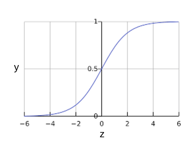
Figure 1: Sigmoid function.
If $z$ represents the output of the linear layer of a model trained with logistic regression, then $sigmoid(z)$ will yield a value (a probability) between 0 and 1. In mathematical terms:
$$y^ \prime = \dfrac{1}{1 + e^{-z}}$$
where:
- $y^ \prime$ is the output of the logistic regression model for a particular example.
For $z$:
where:
- The $w$ values are the model's learned weights, and $b$ is the bias.
- The $x$ values are the feature values for a particular example.
Note that $z$ is also referred to as the log-odds because the inverse of the sigmoid states that $z$ can be defined as the log of the probability of the 1 label (eg., "dog barks") divided by the probability of the 0 label (eg., "dog doesn't bark"):
$$z = \mathrm{log} \left( \dfrac{y}{1- y} \right)$$
Here is the sigmoid function with ML labels:

Figure 2: Logistic regression output.
Loss and Regularization
Loss function for Logistic Regression
The loss function for linear regression is squared loss. The loss function for logistic regression is Log Loss, which is defined as follows:
where:
- $(x,y) \in D$ is the data set containing many labeled examples, which are $(x,y)$ pairs.
- $y$ is the label in a labeled example. Since this is logistic regression, every value of $y$ must either be 0 or 1.
- $y^ \prime$ is the predicted value (somewhere between 0 and 1), given the set of features in $x$.
Regularization in Logistic Regression
Regularization is extremely important in logistic regression modeling. Without regularization, the asymptotic nature of logistic regression would keep driving loss towards 0 in high dimensions. Consequently, most logistic regression models use one of the following two strategies to dampen model complexity:
- $L_{2}$ regularization
- Early stopping, that is, limiting the number of training steps or the learning rate.
Imagine that you assign a unique id to each example, and map each id to its own feature. If you don't specify a regularization function, the model will become completely overfit. That's because the model would try to drive loss to zero on all examples and never get there, driving the weights for each indicator feature to +infinity or -infinity. This can happen in high dimensional data with feature crosses, when there’s a huge mass of rare crosses that happen only on one example each.
Fortunately, using L2 or early stopping will prevent this problem.
Classification
Thresholding
Logistic regression returns a probability. You can use the returned probability "as is" (for example, the probability that the user will click on this ad is 0.00023) or convert the returned probability to a binary value (for example, this email is spam).
A logistic regression model that returns 0.9995 for a particular email message is predicting that it is very likely to be spam. Conversely, another email message with a prediction score of 0.0003 on that same logistic regression model is very likely not spam. However, what about an email message with a prediction score of 0.6? In order to map a logistic regression value to a binary category, you must define a classification threshold (also called the decision threshold). A value above that threshold indicates "spam"; a value below indicates "not spam." It is tempting to assume that the classification threshold should always be 0.5, but thresholds are problem-dependent, and are therefore values that you must tune.
True vs. False and Positive vs. Negative
In this section, we'll define the primary building blocks of the metrics we'll use to evaluate classification models. But first, a fable:
An Aesop's Fable: The Boy Who Cried Wolf (compressed)
A shepherd boy gets bored tending the town's flock. To have some fun, he cries out, "Wolf!" even though no wolf is in sight. The villagers run to protect the flock, but then get really mad when they realize the boy was playing a joke on them.
[Iterate previous paragraph N times.]
One night, the shepherd boy sees a real wolf approaching the flock and calls out, "Wolf!" The villagers refuse to be fooled again and stay in their houses. The hungry wolf turns the flock into lamb chops. The town goes hungry. Panic ensues.
Let's make the following definitions:
- "Wolf" is a positive class.
- "No wolf" is a negative class.
We can summarize our "wolf-prediction" model using a 2x2 confusion matrix that depicts all four possible outcomes:
True Positive (TP):
- Reality: A wolf threatened.
- Shepherd said: "Wolf."
- Outcome: Shepherd is a hero.
False Positive (FP):
- Reality: No wolf threatened.
- Shepherd said: "Wolf."
- Outcome: Villagers are angry at shepherd for waking them up.
True Negative (TN):
- Reality: No wolf threatened.
- Shepherd said: "No wolf."
- Outcome: Everyone is fine.
False Negative (FN):
- Reality: A wolf threatened.
- Shepherd said: "No wolf."
- Outcome: The wolf ate all the sheep.
A true positive is an outcome where the model correctly predicts the positive class. Similarly, a true negative is an outcome where the model correctly predicts the negative class.
A false positive is an outcome where the model incorrectly predicts the positive class. And a false negative is an outcome where the model incorrectly predicts the negative class.
Accuracy
Accuracy is one metric for evaluating classification models. Informally, accuracy is the fraction of predictions our model got right. Formally, accuracy has the following definition:
For binary classification, accuracy can also be calculated in terms of positives and negatives as follows:
Where TP = True Positives, TN = True Negatives, FP = False Positives, and FN = False Negatives.
Let's try calculating accuracy for the following model that classified 100 tumors as malignant (the positive class) or benign (the negative class):
True Positive (TP):
- Reality: Malignant
- ML model predicted: Malignant
- Number of TP results: 1
False Positive (FP):
- Reality: Benign
- ML model predicted: Malignant
- Number of TP results: 1
True Negative (TN):
- Reality: Benign
- ML model predicted: Benign
- Number of TP results: 90
False Negative (FN):
- Reality: Malignant
- ML model predicted: Benign
- Number of TP results: 8
Accuracy comes out to 0.91, or 91% (91 correct predictions out of 100 total examples). That means our tumor classifier is doing a great job of identifying malignancies, right?
Actually, let's do a closer analysis of positives and negatives to gain more insight into our model's performance.
Of the 100 tumor examples, 91 are benign (90 TNs and 1 FP) and 9 are malignant (1 TP and 8 FNs).
Of the 91 benign tumors, the model correctly identifies 90 as benign. That's good. However, of the 9 malignant tumors, the model only correctly identifies 1 as malignant—a terrible outcome, as 8 out of 9 malignancies go undiagnosed!
While 91% accuracy may seem good at first glance, another tumor-classifier model that always predicts benign would achieve the exact same accuracy (91/100 correct predictions) on our examples. In other words, our model is no better than one that has zero predictive ability to distinguish malignant tumors from benign tumors.
Accuracy alone doesn't tell the full story when you're working with a class-imbalanced data set, like this one, where there is a significant disparity between the number of positive and negative labels.
Precision and Recall
Precision
Precision attempts to answer the following question:
What proportion of positive identifications was actually correct?
Precision is defined as follows:
Let's calculate precision for our ML model from the previous section that analyzes tumors:
- True Positives (TPs): 1
- False Positives (FPs): 1
- False Negatives (FNs): 8
- True Negatives (TNs): 90
Our model has a precision of 0.5—in other words, when it predicts a tumor is malignant, it is correct 50% of the time.
Recall
Recall attempts to answer the following question:
What proportion of actual positives was identified correctly?
Mathematically, recall is defined as follows:
$\mathrm{Recall} = \dfrac{TP}{TP + FN}$
Let's calculate recall for our tumor classifier:
- True Positives (TPs): 1
- False Positives (FPs): 1
- False Negatives (FNs): 8
- True Negatives (TNs): 90
Our model has a recall of 0.11—in other words, it correctly identifies 11% of all malignant tumors.
Precision and Recall: A Tug of War
To fully evaluate the effectiveness of a model, you must examine both precision and recall. Unfortunately, precision and recall are often in tension. That is, improving precision typically reduces recall and vice versa. Explore this notion by looking at the following figure, which shows 30 predictions made by an email classification model. Those to the right of the classification threshold are classified as "spam", while those to the left are classified as "not spam."

Figure 1. Classifying email messages as spam or not spam.
Let's calculate precision and recall based on the results shown in Figure 1:
- True Positives (TP): 8
- False Positives (FP): 2
- False Negatives (FN): 3
- True Negatives (TN): 17
Precision measures the percentage of emails flagged as spam that were correctly classified—that is, the percentage of dots to the right of the threshold line that are green in Figure 1:
Recall measures the percentage of actual spam emails that were correctly classified—that is, the percentage of green dots that are to the right of the threshold line in Figure 1:
Figure 2 illustrates the effect of increasing the classification threshold.

Figure 2. Increasing classification threshold.
The number of false positives decreases, but false negatives increase. As a result, precision increases, while recall decreases:
- True Positives (TP): 7
- False Positives (FP): 1
- False Negatives (FN): 4
- True Negatives (TN): 18
Conversely, Figure 3 illustrates the effect of decreasing the classification threshold (from its original position in Figure 1).

Figure 3. Decreasing classification threshold.
False positives increase, and false negatives decrease. As a result, this time, precision decreases and recall increases:
- True Positives (TP): 9
- False Positives (FP): 3
- False Negatives (FN): 2
- True Negatives (TN): 16
Various metrics have been developed that rely on both precision and recall. For example, see F1 score.
ROC Curve and AUC
ROC Curve
An ROC curve (receiver operating characteristic curve) is a graph showing the performance of a classification model at all classification thresholds. This curve plots two parameters:
- True positive rate
- False positive rate
True Positive Rate (TPR) is a synonym for recall and is therefore defined as follows:
$\mathrm{TPR} = \dfrac{TP}{TP + FN}$
False Positive Rate (FPR) is defined as follows:
$\mathrm{FPR} = \dfrac{FP}{FP + TN}$
An ROC curve plots TPR vs. FPR at different classification thresholds. Lowering the classification threshold classifies more items as positive, thus increasing both False Positives and True Positives. The following figure shows a typical ROC curve.

Figure 4. TP vs. FP rate at different classification thresholds.
To compute the points in an ROC curve, we could evaluate a logistic regression model many times with different classification thresholds, but this would be inefficient. Fortunately, there's an efficient, sorting-based algorithm that can provide this information for us, called AUC.
AUC: Area Under the ROC Curve
AUC stands for "Area under the ROC Curve." That is, AUC measures the entire two-dimensional area underneath the entire ROC curve (think integral calculus) from (0,0) to (1,1).

Figure 5. AUC (Area under the ROC Curve).
AUC provides an aggregate measure of performance across all possible classification thresholds. One way of interpreting AUC is as the probability that the model ranks a random positive example more highly than a random negative example. For example, given the following examples, which are arranged from left to right in ascending order of logistic regression predictions:

Figure 6. Predictions ranked in ascending order of logistic regression score.
AUC represents the probability that a random positive (green) example is positioned to the right of a random negative (red) example.
AUC ranges in value from 0 to 1. A model whose predictions are 100% wrong has an AUC of 0.0; one whose predictions are 100% correct has an AUC of 1.0.
AUC is desirable for the following two reasons:
- AUC is scale-invariant. It measures how well predictions are ranked, rather than their absolute values.
- AUC is classification-threshold-invariant. It measures the quality of the model's predictions irrespective of what classification threshold is chosen.
However, both these reasons come with caveats, which may limit the usefulness of AUC in certain use cases:
Scale invariance is not always desirable. For example, sometimes we really do need well calibrated probability outputs, and AUC won’t tell us about that.
Classification-threshold invariance is not always desirable. In cases where there are wide disparities in the cost of false negatives vs. false positives, it may be critical to minimize one type of classification error. For example, when doing email spam detection, you likely want to prioritize minimizing false positives (even if that results in a significant increase of false negatives). AUC isn't a useful metric for this type of optimization.
Prediction Bias
Logistic regression predictions should be unbiased. That is:
"average of predictions" should ≈ "average of observations"
Prediction bias is a quantity that measures how far apart those two averages are. That is:
Note: "Prediction bias" is a different quantity than bias (the b in wx + b).
A significant nonzero prediction bias tells you there is a bug somewhere in your model, as it indicates that the model is wrong about how frequently positive labels occur.
For example, let's say we know that on average, 1% of all emails are spam. If we don't know anything at all about a given email, we should predict that it's 1% likely to be spam. Similarly, a good spam model should predict on average that emails are 1% likely to be spam. (In other words, if we average the predicted likelihoods of each individual email being spam, the result should be 1%.) If instead, the model's average prediction is 20% likelihood of being spam, we can conclude that it exhibits prediction bias.
Possible root causes of prediction bias are:
- Incomplete feature set
- Noisy data set
- Buggy pipeline
- Biased training sample
- Overly strong regularization
You might be tempted to correct prediction bias by post-processing the learned model—that is, by adding a calibration layer that adjusts your model's output to reduce the prediction bias. For example, if your model has +3% bias, you could add a calibration layer that lowers the mean prediction by 3%. However, adding a calibration layer is a bad idea for the following reasons:
- You're fixing the symptom rather than the cause.
- You've built a more brittle system that you must now keep up to date.
If possible, avoid calibration layers. Projects that use calibration layers tend to become reliant on them—using calibration layers to fix all their model's sins. Ultimately, maintaining the calibration layers can become a nightmare.
Note: A good model will usually have near-zero bias. That said, a low prediction bias does not prove that your model is good. A really terrible model could have a zero prediction bias. For example, a model that just predicts the mean value for all examples would be a bad model, despite having zero bias.
Bucketing and Prediction Bias
Logistic regression predicts a value between 0 and 1. However, all labeled examples are either exactly 0 (meaning, for example, "not spam") or exactly 1 (meaning, for example, "spam"). Therefore, when examining prediction bias, you cannot accurately determine the prediction bias based on only one example; you must examine the prediction bias on a "bucket" of examples. That is, prediction bias for logistic regression only makes sense when grouping enough examples together to be able to compare a predicted value (for example, 0.392) to observed values (for example, 0.394).
You can form buckets in the following ways:
- Linearly breaking up the target predictions.
- Forming quantiles.
Consider the following calibration plot from a particular model. Each dot represents a bucket of 1,000 values. The axes have the following meanings:
- The x-axis represents the average of values the model predicted for that bucket.
- The y-axis represents the actual average of values in the data set for that bucket.
Both axes are logarithmic scales.

Figure 8. Prediction bias curve (logarithmic scales)
Why are the predictions so poor for only part of the model? Here are a few possibilities:
- The training set doesn't adequately represent certain subsets of the data space.
- Some subsets of the data set are noisier than others.
- The model is overly regularized. (Consider reducing the value of lambda.)
Regularization for Sparsity
L₁ Regularization
Sparse vectors often contain many dimensions. Creating a feature cross results in even more dimensions. Given such high-dimensional feature vectors, model size may become huge and require huge amounts of RAM.
In a high-dimensional sparse vector, it would be nice to encourage weights to drop to exactly 0 where possible. A weight of exactly 0 essentially removes the corresponding feature from the model. Zeroing out features will save RAM and may reduce noise in the model.
For example, consider a housing data set that covers not just California but the entire globe. Bucketing global latitude at the minute level (60 minutes per degree) gives about 10,000 dimensions in a sparse encoding; global longitude at the minute level gives about 20,000 dimensions. A feature cross of these two features would result in roughly 200,000,000 dimensions. Many of those 200,000,000 dimensions represent areas of such limited residence (for example, the middle of the ocean) that it would be difficult to use that data to generalize effectively. It would be silly to pay the RAM cost of storing these unneeded dimensions. Therefore, it would be nice to encourage the weights for the meaningless dimensions to drop to exactly 0, which would allow us to avoid paying for the storage cost of these model coefficients at inference time.
We might be able to encode this idea into the optimization problem done at training time, by adding an appropriately chosen regularization term.
Would $L_{2}$ regularization accomplish this task? Unfortunately not. $L_{2}$ regularization encourages weights to be small, but doesn't force them to exactly 0.0.
An alternative idea would be to try and create a regularization term that penalizes the count of non-zero coefficient values in a model. Increasing this count would only be justified if there was a sufficient gain in the model's ability to fit the data. Unfortunately, while this count-based approach is intuitively appealing, it would turn our convex optimization problem into a non-convex optimization problem. So this idea, known as $L_{0}$ regularization isn't something we can use effectively in practice.
However, there is a regularization term called $L_{1}$ regularization that serves as an approximation to $L_{0}$, but has the advantage of being convex and thus efficient to compute. So we can use $L_{1}$ regularization to encourage many of the uninformative coefficients in our model to be exactly 0, and thus reap RAM savings at inference time.
$L_{1}$ vs. $L_{2}$ regularization
$L_{2}$ and $L_{1}$ penalize weights differently:
- $L_{2}$ penalizes $weight^2$.
- $L_{1}$ penalizes $|weight|$.
Consequently, $L_{2}$ and $L_{1}$ have different derivatives:
- The derivative of $L_{2}$ is 2 * weight.
- The derivative of $L_{1}$ is k (a constant, whose value is independent of weight).
You can think of the derivative of $L_{2}$ as a force that removes x% of the weight every time. As Zeno knew, even if you remove x percent of a number billions of times, the diminished number will still never quite reach zero. (Zeno was less familiar with floating-point precision limitations, which could possibly produce exactly zero.) At any rate, $L_{2}$ does not normally drive weights to zero.
You can think of the derivative of $L_{1}$ as a force that subtracts some constant from the weight every time. However, thanks to absolute values, $L_{1}$ has a discontinuity at 0, which causes subtraction results that cross 0 to become zeroed out. For example, if subtraction would have forced a weight from +0.1 to -0.2, $L_{1}$ will set the weight to exactly 0. Eureka, $L_{1}$ zeroed out the weight.
$L_{1}$ regularization—penalizing the absolute value of all the weights—turns out to be quite efficient for wide models.
Note that this description is true for a one-dimensional model.
To compare the results of $L_{1}$ and $L_{2}$ regularization on a network of weights, click the play button on the playground.
Neural Networks
Neural networks are a more sophisticated version of feature crosses. In essence, neural networks learn the appropriate feature crosses for you.
Structure
If you recall from the Feature Crosses unit, the following classification problem is nonlinear:
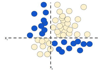
Figure 1. Nonlinear classification problem.
"Nonlinear" means that you can't accurately predict a label with a model of the form $b + w_{1}x_{1} + w_{2}x_{2}$ In other words, the "decision surface" is not a line. Previously, we looked at feature crosses as one possible approach to modeling nonlinear problems.
Now consider the following data set:
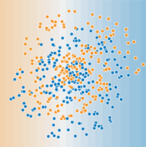
Figure 2. A more difficult nonlinear classification problem.
The data set shown in Figure 2 can't be solved with a linear model.
To see how neural networks might help with nonlinear problems, let's start by representing a linear model as a graph:

Figure 3. Linear model as graph.
Each blue circle represents an input feature, and the green circle represents the weighted sum of the inputs.
The Linear Unit
So let's begin with the fundamental component of a neural network: the individual neuron. As a diagram, a neuron (or unit) with one input looks like:
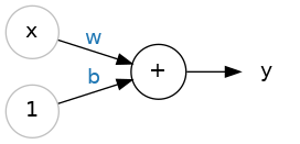
The Linear Unit: y = wx + b
The input is $x$. Its connection to the neuron has a weight which is $w$. Whenever a value flows through a connection, you multiply the value by the connection's weight. For the input $x$, what reaches the neuron is $w * x$. A neural network "learns" by modifying its weights.
The $b$ is a special kind of weight we call it bias. The bias doesn't have any input data associated with it; instead, we put a $1$ in the diagram so that the value that reaches the neuron is just $b$ (since $1 * b = b$). The bias enables the neuron to modify the output independently of its inputs.
The $y$ is the value the neuron ultimately outputs. To get the output, the neuron sums up all the values it receives through its connections. This neuron's activation is $y = w * x + b$, or as a formula $y=wx+b$.
Multiple Inputs
In the previous section we saw how can we handle a single input using The Linear Unit, but what if we wanted to expand our model to include more inputs? That's easy enough. We can just add more input connections to the neuron, one for each additional feature. To find the output, we would multiply each input to its connection weight and then add them all together.
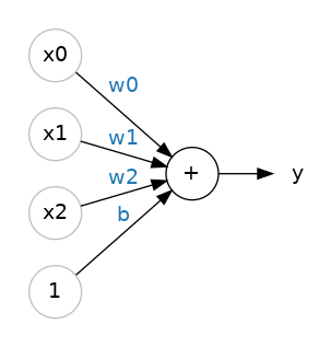
A linear unit with three inputs.
The formula for this neuron would be $y=w0x0+w1x1+w2x2+b$. A linear unit with two inputs will fit a plane, and a unit with more inputs than that will fit a hyperplane.
Layers
Neural networks typically organize their neurons into layers. When we collect together linear units having a common set of inputs we get a dense layer.

A dense layer of two linear units receiving two inputs and a bias.
You could think of each layer in a neural network as performing some kind of relatively simple transformation. Through a deep stack of layers, a neural network can transform its inputs in more and more complex ways. In a well-trained neural network, each layer is a transformation getting us a little bit closer to a solution.
Hidden Layers
In the model represented by the following graph, we've added a "hidden layer" of intermediary values. Each yellow node in the hidden layer is a weighted sum of the blue input node values. The output is a weighted sum of the yellow nodes.

Figure 4. Graph of two-layer model.
Is this model linear? Yes—its output is still a linear combination of its inputs.
In the model represented by the following graph, we've added a second hidden layer of weighted sums.

Figure 5. Graph of three-layer model.
Is this model still linear? Yes, it is. When you express the output as a function of the input and simplify, you get just another weighted sum of the inputs. This sum won't effectively model the nonlinear problem in Figure 2.
Activation Functions
 Without activation functions, neural networks can only learn linear relationships. In order to fit curves, we'll need to use activation functions.
To model a nonlinear problem, we can directly introduce a nonlinearity. We can pipe each hidden layer node through a nonlinear function.
In the model represented by the following graph, the value of each node in Hidden Layer 1 is transformed by a nonlinear function before being passed on to the weighted sums of the next layer. This nonlinear function is called the activation function.

Figure 6. Graph of three-layer model with activation function.
An activation function is simply some function we apply to each of a layer's outputs (its activations). The most common is the rectifier function $max(0,x)$.

The rectifier function has a graph that's a line with the negative part "rectified" to zero. Applying the function to the outputs of a neuron will put a bend in the data, moving us away from simple lines.
When we attach the rectifier to a linear unit, we get a rectified linear unit or ReLU. (For this reason, it's common to call the rectifier function the "ReLU function".) Applying a ReLU activation to a linear unit means the output becomes $max(0, w * x + b)$, which we might draw in a diagram like:
 A rectified linear unit.
Now that we've added an activation function, adding layers has more impact. Stacking nonlinearities on nonlinearities lets us model very complicated relationships between the inputs and the predicted outputs. In brief, each layer is effectively learning a more complex, higher-level function over the raw inputs. If you'd like to develop more intuition on how this works, see Chris Olah's excellent blog post.
Common Activation Functions
The following sigmoid activation function converts the weighted sum to a value between 0 and 1.
$$F(x)=\dfrac{1}{1 + e^{-x}}$$
Here's a plot:

Figure 7. Sigmoid activation function.
The following rectified linear unit activation function (or ReLU, for short) often works a little better than a smooth function like the sigmoid, while also being significantly easier to compute.
$$F(x) = max(0, x)$$
The superiority of ReLU is based on empirical findings, probably driven by ReLU having a more useful range of responsiveness. A sigmoid's responsiveness falls off relatively quickly on both sides.

Figure 8. ReLU activation function.
In fact, any mathematical function can serve as an activation function. Suppose that $\sigma$ represents our activation function (Relu, Sigmoid, or whatever). Consequently, the value of a node in the network is given by the following formula:
$$\sigma(w.x + b)$$
TensorFlow provides out-of-the-box support for many activation functions. You can find these activation functions within TensorFlow's list of wrappers for primitive neural network operations. That said, we still recommend starting with ReLU.
Stacking Dense Layers
Now that we have some nonlinearity, let's see how we can stack layers to get complex data transformations.
 A stack of dense layers makes a "fully-connected" network.
The layers before the output layer are sometimes called hidden since we never see their outputs directly.
Now, notice that the final (output) layer is a linear unit (meaning, no activation function). That makes this network appropriate to a regression task, where we are trying to predict some arbitrary numeric value. Other tasks (like classification) might require an activation function on the output.
Summary
Now our model has all the standard components of what people usually mean when they say "neural network":
- A set of nodes, analogous to neurons, organized in layers.
- A set of weights representing the connections between each neural network layer and the layer beneath it. The layer beneath may be another neural network layer, or some other kind of layer.
- A set of biases, one for each node.
- An activation function that transforms the output of each node in a layer. Different layers may have different activation functions.
Training Neural Networks
Backpropagation is the most common training algorithm for neural networks. It makes gradient descent feasible for multi-layer neural networks.
Best Practices
This section explains backpropagation's failure cases and the most common way to regularize a neural network.
Failure Cases
There are a number of common ways for backpropagation to go wrong.
Vanishing Gradients
The gradients for the lower layers (closer to the input) can become very small. In deep networks, computing these gradients can involve taking the product of many small terms.
When the gradients vanish toward 0 for the lower layers, these layers train very slowly, or not at all.
The ReLU activation function can help prevent vanishing gradients.
Exploding Gradients
If the weights in a network are very large, then the gradients for the lower layers involve products of many large terms. In this case you can have exploding gradients: gradients that get too large to converge.
Batch normalization can help prevent exploding gradients, as can lowering the learning rate.
Dead ReLU Units
Once the weighted sum for a ReLU unit falls below 0, the ReLU unit can get stuck. It outputs 0 activation, contributing nothing to the network's output, and gradients can no longer flow through it during backpropagation. With a source of gradients cut off, the input to the ReLU may not ever change enough to bring the weighted sum back above 0.
Lowering the learning rate can help keep ReLU units from dying.
Dropout Regularization
Yet another form of regularization, called Dropout, is useful for neural networks. It works by randomly "dropping out" unit activations in a network for a single gradient step. The more you drop out, the stronger the regularization:
- 0.0 = No dropout regularization.
- 1.0 = Drop out everything. The model learns nothing.
- Values between 0.0 and 1.0 = More useful.
 Here, 50% dropout has been added between the two hidden layers.
Batch Normalization (batchnorm)
With neural networks, it's generally a good idea to put all of your data on a common scale. The reason is that SGD will shift the network weights in proportion to how large an activation the data produces. Features that tend to produce activations of very different sizes can make for unstable training behavior.
Now, if it's good to normalize the data before it goes into the network, maybe also normalizing inside the network would be better! In fact, we have a special kind of layer that can do this, the batch normalization layer. A batch normalization layer looks at each batch as it comes in, first normalizing the batch with its own mean and standard deviation, and then also putting the data on a new scale with two trainable rescaling parameters. Batchnorm, in effect, performs a kind of coordinated rescaling of its inputs.
Most often, batchnorm is added as an aid to the optimization process (though it can sometimes also help prediction performance). Models with batchnorm tend to need fewer epochs to complete training. Moreover, batchnorm can also fix various problems that can cause the training to get "stuck". Consider adding batch normalization to your models, especially if you're having trouble during training.
  1# Copyright 2023 The AI Authors. All Rights Reserved.
  2#
  3# Licensed under the Apache License, Version 2.0 (the "License");
  4# you may not use this file except in compliance with the License.
  5# You may obtain a copy of the License at
  6#
  7#     http://www.apache.org/licenses/LICENSE-2.0
  8#
  9# Unless required by applicable law or agreed to in writing, software
 10# distributed under the License is distributed on an "AS IS" BASIS,
 11# WITHOUT WARRANTIES OR CONDITIONS OF ANY KIND, either express or implied.
 12# See the License for the specific language governing permissions and
 13# limitations under the License.
 14
 15from typing import Union, List
 16
 17import os
 18import pathlib
 19import base64
 20
 21from bs4 import BeautifulSoup
 22from urllib.parse import urlparse
 23
 24from . import stats
 25from . import boolalg
 26from . import neighbors
 27from . import naive_bayes
 28from . import linear_model
 29
 30_DOCS_DIR = pathlib.Path(
 31  os.fspath(os.path.normpath(__file__))
 32).parent.parent / 'docs'
 33_ML_DOCS_DIR = _DOCS_DIR / 'ml'
 34
 35
 36def _ConvertImagePath2Base64(soup: BeautifulSoup) -> BeautifulSoup:
 37  for img in soup.find_all('img'):
 38    src = img.get('src')
 39
 40    if urlparse(src).scheme == '':
 41      with open(src, 'rb') as img_f:
 42        base64_img = base64.b64encode(img_f.read()).decode('utf-8')
 43      img['src'] = f'data:image/png;base64,{base64_img}'
 44  return soup
 45
 46
 47def _WrapImgStrongWithBlock(soup: BeautifulSoup) -> BeautifulSoup:
 48  for img in soup.find_all('img'):
 49    if img.parent.find_all('strong'):
 50      img.parent.strong.wrap(soup.new_tag('p'))
 51  return soup
 52
 53
 54def _MarkdownPreprocessPipeline(
 55  soup: BeautifulSoup, pipeline: List[callable]
 56) -> BeautifulSoup:
 57  for call in pipeline:
 58    soup = call(soup)
 59  return soup
 60
 61
 62def _PreprocessReadme(fpath: Union[str, pathlib.Path]) -> str:
 63  with open(fpath, mode='r', encoding='utf-8') as f:
 64    readme = f.read()
 65
 66  soup = BeautifulSoup(readme, 'html.parser')
 67  soup = _MarkdownPreprocessPipeline(
 68    soup, (_ConvertImagePath2Base64, _WrapImgStrongWithBlock)
 69  )
 70  return str(soup)
 71
 72
 73# DO NOT TOUCH! THIS KEEPS THE DOCUMENTATION IN ORDER!
 74_ML_README_FILES = (
 75  'Introduction-to-ML.md',
 76  'Descending-into-ML.md',
 77  'Reducing-Loss.md',
 78  'Generalization.md',
 79  'Training-and-Test-Sets.md',
 80  'Validation-Set.md',
 81  'Representation.md',
 82  'Feature-Crosses.md',
 83  'Transform-Your-Data.md',
 84  'Regularization-for-Simplicity.md',
 85  'Logistic-Regression.md',
 86  'Classification.md',
 87  'Regularization-for-Sparsity.md',
 88  'Neural-Networks.md',
 89  'Training-Neural-Networks.md',
 90)
 91
 92
 93def _MakeDocs(docs_dir: pathlib.Path) -> str:
 94  doc = ''
 95  for readme in _ML_README_FILES:
 96    doc += _PreprocessReadme(_ML_DOCS_DIR / readme)
 97  return doc
 98
 99
100__doc__ = _MakeDocs(_ML_DOCS_DIR)