Descending into ML¶

Linear regression is a method for finding the straight line or hyperplane that best fits a set of points.

Linear Regression¶

It has long been known that crickets (an insect species) chirp more frequently on hotter days than on cooler days. For decades, professional and amateur scientists have cataloged data on chirps-per-minute and temperature. As a birthday gift, your Aunt Ruth gives you her cricket database and asks you to learn a model to predict this relationship. Using this data, you want to explore this relationship.

First, examine your data by plotting it:

Figure 1. Chirps per Minute vs. Temperature in Celsius.

As expected, the plot shows the temperature rising with the number of chirps. Is this relationship between chirps and temperature linear? Yes, you could draw a single straight line like the following to approximate this relationship:

Figure 2. A linear relationship.

True, the line doesn't pass through every dot, but the line does clearly show the relationship between chirps and temperature. Using the equation for a line, you could write down this relationship as follows:

\[y=mx+b\]

where:

$y$ is the temperature in Celsius — the value we're trying to predict.
$m$ is the slope of the line.
$x$ is the number of chirps per minute — the value of our input feature.
$b$ is the y-intercept.

By convention in machine learning, you'll write the equation for a model slightly differently:

\[y^\prime=b+w_{1}x_{1}\]

where:

$y^\prime$ is a predicted label (a desired output).
$b$ is the bias (the y-intercept), sometimes referred to as $w_{0}$.
$w_{1}$ is the weight of feature 1. Weight is the same concept as the "slope" $m$ in the traditional equation of a line.
$x_{1}$ is a feature (a known input).

To infer (predict) the temprature $y^\prime$ for new chirps-per-minute value $x_{1}$, just substitute the $x_{1}$ value into this model.

Although this model uses only one feature, a more sophisticated model might rely on multiple features, each having a separate weight ($w_{1}$, $w_{2}$, etc.). For example, a model that relies on three features might look as follows:

\[y^\prime=b+w_{1}x_{1}+w_{2}x_{2}+w_{3}x_{3}\]

Training and Loss¶

Training a model simply means learning (determining) good values for all the weights and the bias from labeled examples. In supervised learning, a machine learning algorithm builds a model by examining many examples and attempting to find a model that minimizes loss; this process is called empirical risk minimization.

Loss is the penalty for a bad prediction. That is, loss is a number indicating how bad the model's prediction was on a single example. If the model's prediction is perfect, the loss is zero; otherwise, the loss is greater. The goal of training a model is to find a set of weights and biases that have low loss, on average, across all examples. For example, Figure 3 shows a high loss model on the left and a low loss model on the right. Note the following about the figure:

The arrows represent loss.
The blue lines represent predictions.

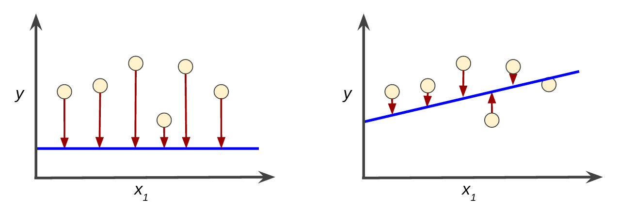Figure 3. High loss in the left model; low loss in the right model.

Notice that the arrows in the left plot are much longer than their counterparts in the right plot. Clearly, the line in the right plot is a much better predictive model than the line in the left plot.

You might be wondering whether you could create a mathematical function — a loss function — that would aggregate the individual losses in a meaningful fashion.

Squared loss: a popular loss function¶

The linear regression models we'll examine here use a loss function called squared loss (also known as L2 loss). The squared loss for a single example is as follows:

  = the square of the difference between the label and the prediction
  = (observation - prediction(x))2
  = (y - y')2

Mean square error (MSE) is the average squared loss per example over the whole dataset. To calculate MSE, sum up all the squared losses for individual examples and then divide by the number of examples:

$$\mathrm{MSE}=\dfrac{1}{N}\sum_{(x,y) \in D} (y - \mathrm{prediction}(x))^2$$

where:

$(x,y)$ is an example in which
$x$ is a set of features (for example chirps/minute, age, gender) that the model uses to make predictions.
$y$ is the example's label (for example, temprature).
$prediction(x)$ is a function of the weights and bias in combination with the sets of features $x$.
$D$ is a dataset containing many labeled examples, which are $(x,y)$ pairs.
$N$ is the number of examples in $D$.

Although MSE is commonly-used in machine learning, it is neither the only practical loss function nor the best loss function for all circumstances.