Feature Crosses
A feature cross is a synthetic feature formed by multiplying (crossing) two or more features. Crossing combinations of features can provide predictive abilities beyond what those features can provide individually.
Encoding Nonlinearity
In Figures 1 and 2, imagine the following:
- The blue dots represent sick trees.
- The orange dots represent healthy trees.
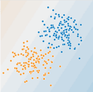 Figure 1. Is this a linear problem?
Can you draw a line that neatly separates the sick trees from the healthy trees? Sure. This is a linear problem. The line won't be perfect. A sick tree or two might be on the "healthy" side, but your line will be a good predictor.
Now look at the following figure:
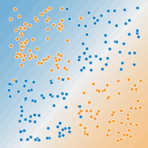 Figure 2. Is this a linear problem?
Can you draw a single straight line that neatly separates the sick trees from the healthy trees? No, you can't. This is a nonlinear problem. Any line you draw will be a poor predictor of tree health.
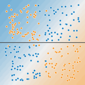 Figure 3. A single line can't separate the two classes.
To solve the nonlinear problem shown in Figure 2, create a feature cross. A feature cross is a synthetic feature that encodes nonlinearity in the feature space by multiplying two or more input features together. (The term cross comes from cross product.) Let's create a feature cross named \(x_{3}\) by crossing \(x_{1}\) and \(x_{2}\):
We treat this newly minted \(x_{3}\) feature cross just like any other feature. The linear formula becomes:
A linear algorithm can learn a weight for \(w_{3}\) just as it would for \(w_{1}\) and \(w_{2}\). In other words, although \(w_{3}\) encodes nonlinear information, you don’t need to change how the linear model trains to determine the value of \(w_{3}\).
Kinds of feature crosses
We can create many different kinds of feature crosses. For example:
[A X B]: a feature cross formed by multiplying the values of two features.[A x B x C x D x E]: a feature cross formed by multiplying the values of five features.[A x A]: a feature cross formed by squaring a single feature.
Thanks to stochastic gradient descent, linear models can be trained efficiently. Consequently, supplementing scaled linear models with feature crosses has traditionally been an efficient way to train on massive-scale data sets.
Crossing One-Hot Vectors
So far, we've focused on feature-crossing two individual floating-point features. In practice, machine learning models seldom cross continuous features. However, machine learning models do frequently cross one-hot feature vectors. Think of feature crosses of one-hot feature vectors as logical conjunctions. For example, suppose we have two features: country and language. A one-hot encoding of each generates vectors with binary features that can be interpreted as country=USA, country=France or language=English, language=Spanish. Then, if you do a feature cross of these one-hot encodings, you get binary features that can be interpreted as logical conjunctions, such as:
As another example, suppose you bin latitude and longitude, producing separate one-hot five-element feature vectors. For instance, a given latitude and longitude could be represented as follows:
Suppose you create a feature cross of these two feature vectors:
This feature cross is a 25-element one-hot vector (24 zeroes and 1 one). The single 1 in the cross identifies a particular conjunction of latitude and longitude. Your model can then learn particular associations about that conjunction.
Suppose we bin latitude and longitude much more coarsely, as follows:
binned_latitude(lat) = [
  0  < lat <= 10
  10 < lat <= 20
  20 < lat <= 30
]

binned_longitude(lon) = [
  0  < lon <= 15
  15 < lon <= 30
]
Creating a feature cross of those coarse bins leads to synthetic feature having the following meanings:
binned_latitude_X_longitude(lat, lon) = [
  0  < lat <= 10 AND 0  < lon <= 15
  0  < lat <= 10 AND 15 < lon <= 30
  10 < lat <= 20 AND 0  < lon <= 15
  10 < lat <= 20 AND 15 < lon <= 30
  20 < lat <= 30 AND 0  < lon <= 15
  20 < lat <= 30 AND 15 < lon <= 30
]
Now suppose our model needs to predict how satisfied dog owners will be with dogs based on two features:
- Behavior type (barking, crying, snuggling, etc.)
- Time of day
If we build a feature cross from both these features:
then we'll end up with vastly more predictive ability than either feature on its own. For example, if a dog cries (happily) at 5:00 pm when the owner returns from work will likely be a great positive predictor of owner satisfaction. Crying (miserably, perhaps) at 3:00 am when the owner was sleeping soundly will likely be a strong negative predictor of owner satisfaction.
Linear learners scale well to massive data. Using feature crosses on massive data sets is one efficient strategy for learning highly complex models. Neural networks provide another strategy.