Neural Networks
Neural networks are a more sophisticated version of feature crosses. In essence, neural networks learn the appropriate feature crosses for you.
Structure
If you recall from the Feature Crosses unit, the following classification problem is nonlinear:
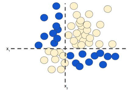 Figure 1. Nonlinear classification problem.
"Nonlinear" means that you can't accurately predict a label with a model of the form \(b + w_{1}x_{1} + w_{2}x_{2}\) In other words, the "decision surface" is not a line. Previously, we looked at feature crosses as one possible approach to modeling nonlinear problems.
Now consider the following data set:
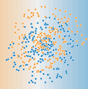 Figure 2. A more difficult nonlinear classification problem.
The data set shown in Figure 2 can't be solved with a linear model.
To see how neural networks might help with nonlinear problems, let's start by representing a linear model as a graph:
 Figure 3. Linear model as graph.
Each blue circle represents an input feature, and the green circle represents the weighted sum of the inputs.
The Linear Unit
So let's begin with the fundamental component of a neural network: the individual neuron. As a diagram, a neuron (or unit) with one input looks like:
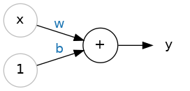 The Linear Unit: y = wx + b
The input is \(x\). Its connection to the neuron has a weight which is \(w\). Whenever a value flows through a connection, you multiply the value by the connection's weight. For the input \(x\), what reaches the neuron is \(w * x\). A neural network "learns" by modifying its weights.
The \(b\) is a special kind of weight we call it bias. The bias doesn't have any input data associated with it; instead, we put a \(1\) in the diagram so that the value that reaches the neuron is just \(b\) (since \(1 * b = b\)). The bias enables the neuron to modify the output independently of its inputs.
The \(y\) is the value the neuron ultimately outputs. To get the output, the neuron sums up all the values it receives through its connections. This neuron's activation is \(y = w * x + b\), or as a formula \(y=wx+b\).
Multiple Inputs
In the previous section we saw how can we handle a single input using The Linear Unit, but what if we wanted to expand our model to include more inputs? That's easy enough. We can just add more input connections to the neuron, one for each additional feature. To find the output, we would multiply each input to its connection weight and then add them all together.
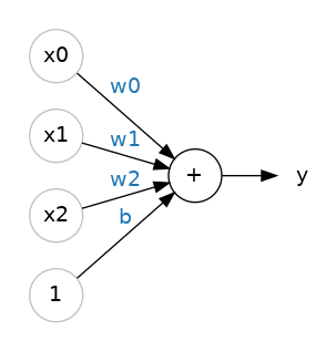 A linear unit with three inputs.
The formula for this neuron would be \(y=w0x0+w1x1+w2x2+b\). A linear unit with two inputs will fit a plane, and a unit with more inputs than that will fit a hyperplane.
Layers
Neural networks typically organize their neurons into layers. When we collect together linear units having a common set of inputs we get a dense layer.
 A dense layer of two linear units receiving two inputs and a bias.
You could think of each layer in a neural network as performing some kind of relatively simple transformation. Through a deep stack of layers, a neural network can transform its inputs in more and more complex ways. In a well-trained neural network, each layer is a transformation getting us a little bit closer to a solution.
Hidden Layers
In the model represented by the following graph, we've added a "hidden layer" of intermediary values. Each yellow node in the hidden layer is a weighted sum of the blue input node values. The output is a weighted sum of the yellow nodes.
 Figure 4. Graph of two-layer model.
Is this model linear? Yes—its output is still a linear combination of its inputs.
In the model represented by the following graph, we've added a second hidden layer of weighted sums.
 Figure 5. Graph of three-layer model.
Is this model still linear? Yes, it is. When you express the output as a function of the input and simplify, you get just another weighted sum of the inputs. This sum won't effectively model the nonlinear problem in Figure 2.
Activation Functions
 Without activation functions, neural networks can only learn linear relationships. In order to fit curves, we'll need to use activation functions.
To model a nonlinear problem, we can directly introduce a nonlinearity. We can pipe each hidden layer node through a nonlinear function.
In the model represented by the following graph, the value of each node in Hidden Layer 1 is transformed by a nonlinear function before being passed on to the weighted sums of the next layer. This nonlinear function is called the activation function.
 Figure 6. Graph of three-layer model with activation function.
An activation function is simply some function we apply to each of a layer's outputs (its activations). The most common is the rectifier function \(max(0,x)\).

The rectifier function has a graph that's a line with the negative part "rectified" to zero. Applying the function to the outputs of a neuron will put a bend in the data, moving us away from simple lines.
When we attach the rectifier to a linear unit, we get a rectified linear unit or ReLU. (For this reason, it's common to call the rectifier function the "ReLU function".) Applying a ReLU activation to a linear unit means the output becomes \(max(0, w * x + b)\), which we might draw in a diagram like:
 A rectified linear unit.
Now that we've added an activation function, adding layers has more impact. Stacking nonlinearities on nonlinearities lets us model very complicated relationships between the inputs and the predicted outputs. In brief, each layer is effectively learning a more complex, higher-level function over the raw inputs. If you'd like to develop more intuition on how this works, see Chris Olah's excellent blog post.
Common Activation Functions
The following sigmoid activation function converts the weighted sum to a value between 0 and 1.
Here's a plot:
 Figure 7. Sigmoid activation function.
The following rectified linear unit activation function (or ReLU, for short) often works a little better than a smooth function like the sigmoid, while also being significantly easier to compute.
The superiority of ReLU is based on empirical findings, probably driven by ReLU having a more useful range of responsiveness. A sigmoid's responsiveness falls off relatively quickly on both sides.
 Figure 8. ReLU activation function.
In fact, any mathematical function can serve as an activation function. Suppose that \(\sigma\) represents our activation function (Relu, Sigmoid, or whatever). Consequently, the value of a node in the network is given by the following formula:
TensorFlow provides out-of-the-box support for many activation functions. You can find these activation functions within TensorFlow's list of wrappers for primitive neural network operations. That said, we still recommend starting with ReLU.
Stacking Dense Layers
Now that we have some nonlinearity, let's see how we can stack layers to get complex data transformations.
 A stack of dense layers makes a "fully-connected" network.
The layers before the output layer are sometimes called hidden since we never see their outputs directly.
Now, notice that the final (output) layer is a linear unit (meaning, no activation function). That makes this network appropriate to a regression task, where we are trying to predict some arbitrary numeric value. Other tasks (like classification) might require an activation function on the output.
Summary
Now our model has all the standard components of what people usually mean when they say "neural network":
- A set of nodes, analogous to neurons, organized in layers.
- A set of weights representing the connections between each neural network layer and the layer beneath it. The layer beneath may be another neural network layer, or some other kind of layer.
- A set of biases, one for each node.
- An activation function that transforms the output of each node in a layer. Different layers may have different activation functions.