Representation
A machine learning model can't directly see, hear, or sense input examples. Instead, you must create a representation of the data to provide the model with a useful vantage point into the data's key qualities. That is, in order to train a model, you must choose the set of features that best represent the data.
Feature Engineering
In traditional programming, the focus is on code. In machine learning projects, the focus shifts to representation. That is, one way developers hone a model is by adding and improving its features.
Mapping Raw Data to Features
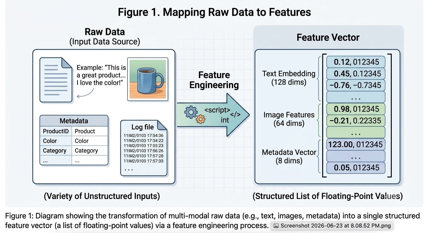
The left side of Figure 1 illustrates raw data from an input data source; the right side illustrates a feature vector, which is the set of floating-point values comprising the examples in your data set. Feature engineering means transforming raw data into a feature vector. Expect to spend significant time doing feature engineering.
Many machine learning models must represent the features as real-numbered vectors since the feature values must be multiplied by the model weights.
Mapping numeric values
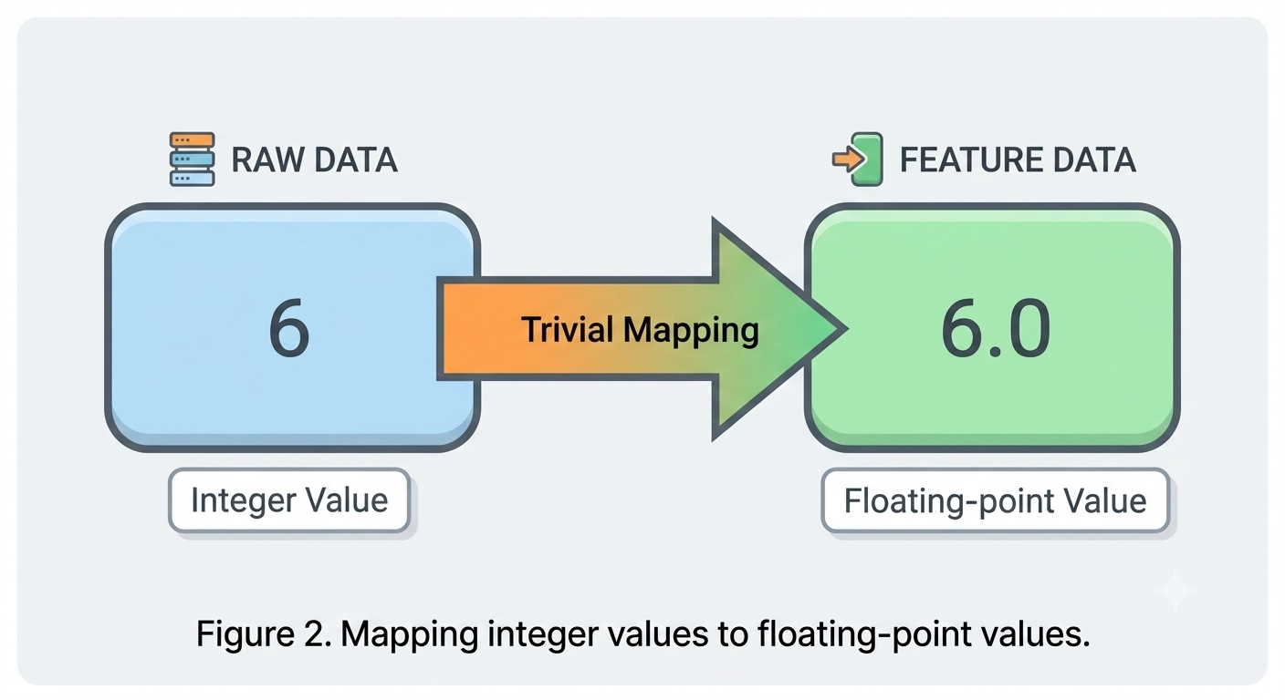
Integer and floating-point data don't need a special encoding because they can be multiplied by a numeric weight. As suggested in Figure 2, converting the raw integer value 6 to the feature value 6.0 is trivial:
Mapping categorical values
Categorical features have a discrete set of possible values. For example, there might be a feature called street_name with options that include:
{'Charleston Road', 'North Shoreline Boulevard', 'Shorebird Way', 'Rengstorff Avenue'}
Since models cannot multiply strings by the learned weights, we use feature engineering to convert strings to numeric values.
We can accomplish this by defining a mapping from the feature values, which we'll refer to as the vocabulary of possible values, to integers. Since not every street in the world will appear in our dataset, we can group all other streets into a catch-all "other" category, known as an OOV (out-of-vocabulary) bucket.
Using this approach, here's how we can map our street names to numbers:
- map Charleston Road to 0
- map North Shoreline Boulevard to 1
- map Shorebird Way to 2
- map Rengstorff Avenue to 3
- map everything else (OOV) to 4
However, if we incorporate these index numbers directly into our model, it will impose some constraints that might be problematic:
- We'll be learning a single weight that applies to all streets. For example, if we learn a weight of 6 for
street_name, then we will multiply it by 0 for Charleston Road, by 1 for North Shoreline Boulevard, 2 for Shorebird Way and so on. Consider a model that predicts house prices usingstreet_nameas a feature. It is unlikely that there is a linear adjustment of price based on the street name, and furthermore this would assume you have ordered the streets based on their average house price. Our model needs the flexibility of learning different weights for each street that will be added to the price estimated using the other features. - We aren't accounting for cases where
street_namemay take multiple values. For example, many houses are located at the corner of two streets, and there's no way to encode that information in thestreet_namevalue if it contains a single index.
To remove both these constraints, we can instead create a binary vector for each categorical feature in our model that represents values as follows:
- For values that apply to the example, set corresponding vector elements to
1. - Set all other elements to
0.
The length of this vector is equal to the number of elements in the vocabulary. This representation is called a one-hot encoding when a single value is 1, and a multi-hot encoding when multiple values are 1.
Figure 3 illustrates a one-hot encoding of a particular street: Shorebird Way. The element in the binary vector for Shorebird Way has a value of 1, while the elements for all other streets have values of 0.
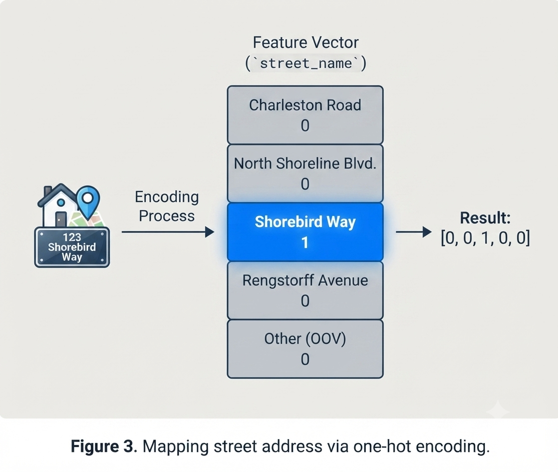
This approach effectively creates a Boolean variable for every feature value (e.g., street name). Here, if a house is on Shorebird Way then the binary value is 1 only for Shorebird Way. Thus, the model uses only the weight for Shorebird Way.
Similarly, if a house is at the corner of two streets, then two binary values are set to 1, and the model uses both their respective weights.
Sparse Representation
Suppose that you had 1,000,000 different street names in your data set that you wanted to include as values for street_name. Explicitly creating a binary vector of 1,000,000 elements where only 1 or 2 elements are true is a very inefficient representation in terms of both storage and computation time when processing these vectors. In this situation, a common approach is to use a sparse representation in which only nonzero values are stored. In sparse representations, an independent model weight is still learned for each feature value, as described above.
Cleaning Data
Apple trees produce some mixture of great fruit and wormy messes. Yet the apples in high-end grocery stores display 100% perfect fruit. Between orchard and grocery, someone spends significant time removing the bad apples or throwing a little wax on the salvageable ones. As an ML engineer, you'll spend enormous amounts of your time tossing out bad examples and cleaning up the salvageable ones. Even a few "bad apples" can spoil a large data set.
Scaling feature values
Scaling means converting floating-point feature values from their natural range (for example, 100 to 900) into a standard range (for example, 0 to 1 or -1 to +1). If a feature set consists of only a single feature, then scaling provides little to no practical benefit. If, however, a feature set consists of multiple features, then feature scaling provides the following benefits:
- Helps gradient descent converge more quickly.
- Helps avoid the "NaN trap," in which one number in the model becomes a NaN (e.g., when a value exceeds the floating-point precision limit during training), and—due to math operations—every other number in the model also eventually becomes a NaN.
- Helps the model learn appropriate weights for each feature. Without feature scaling, the model will pay too much attention to the features having a wider range.
You don't have to give every floating-point feature exactly the same scale. Nothing terrible will happen if Feature A is scaled from -1 to +1 while Feature B is scaled from -3 to +3. However, your model will react poorly if Feature B is scaled from 5000 to 100000.
One obvious way to scale numerical data is to linearly map [min value, max value] to a small scale, such as [-1, +1].
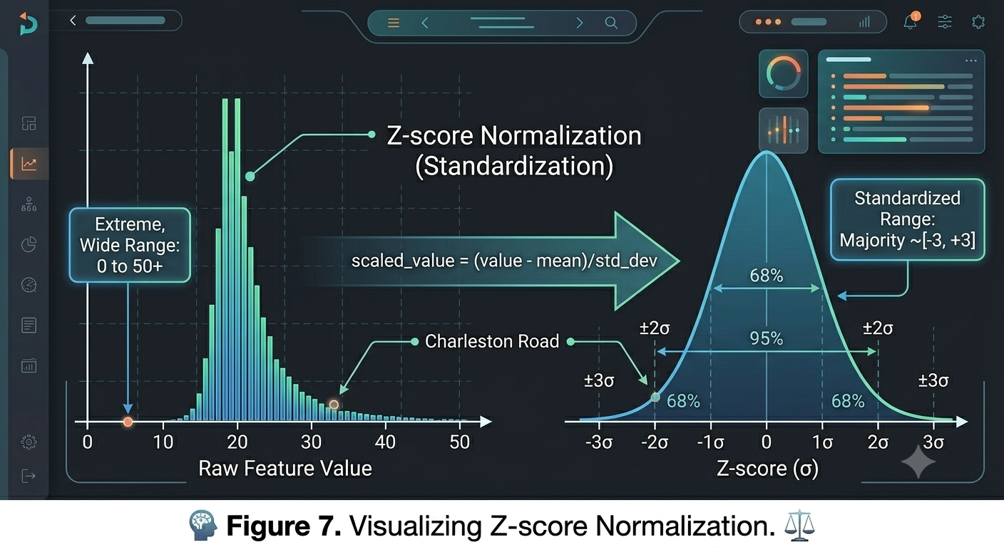
Another popular scaling tactic is to calculate the Z score of each value. The Z score relates the number of standard deviations away from the mean. In other words:
$$\text{scaled value} = (\text{value} - \text{mean})/\text{stddev}$$
For example, given:
- mean = 100
- standard deviation = 20
- original value = 130
then:
scaled_value = (130 - 100) / 20
scaled_value = 1.5
Scaling with Z scores means that most scaled values will be between -3 and +3, but a few values will be a little higher or lower than that range.
Handling extreme outliers
The following plot represents a feature called roomsPerPerson from the California Housing data set. The value of roomsPerPerson was calculated by dividing the total number of rooms for an area by the population for that area. The plot shows that the vast majority of areas in California have one or two rooms per person. But take a look along the x-axis.

How could we minimize the influence of those extreme outliers? Well, one way would be to take the log of every value:
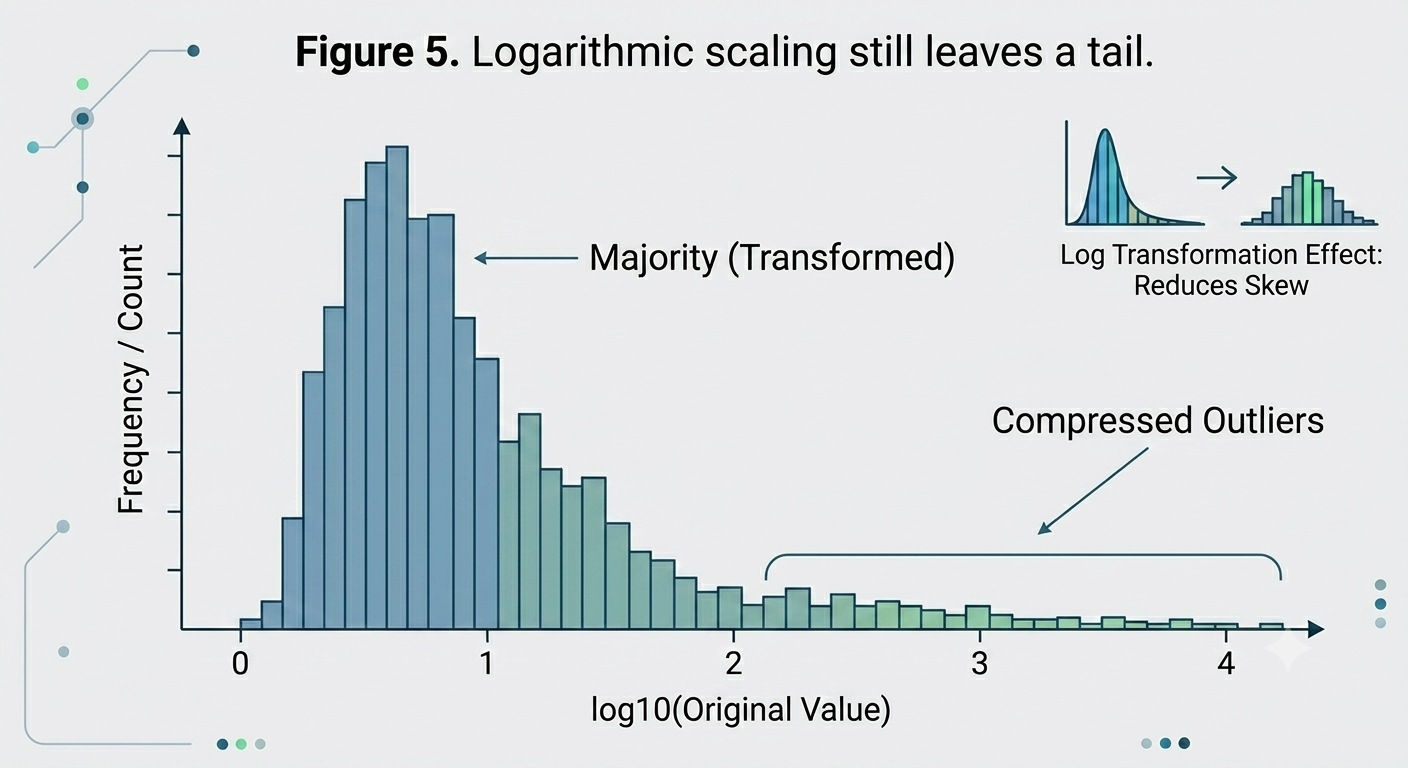
Log scaling does a slightly better job, but there's still a significant tail of outlier values. Let's pick yet another approach. What if we simply "cap" or "clip" the maximum value of roomsPerPerson at an arbitrary value, say 4.0?
Clipping the feature value at 4.0 doesn't mean that we ignore all values greater than 4.0. Rather, it means that all values that were greater than 4.0 now become 4.0. This explains the funny hill at 4.0. Despite that hill, the scaled feature set is now more useful than the original data.