NumPy
Numpy is a Python library for creating and manipulating matrices, the main data structure used by ML algorithms. Matrices are mathematical objects used to store values in rows and columns.
Python calls matrices lists, NumPy calls them arrays and TensorFlow calls them tensors. Python represents matrices with the list data type.
Import NumPy module
Run the following code cell to import the NumPy module:
import numpy as np
Populate arrays with specific numbers
Call np.array to create a NumPy array with your own hand-picked values. For example, the following call to np.array creates an 8-element array:
one_dimensional_array = np.array([1.2, 2.4, 3.5, 4.7, 6.1, 7.2, 8.3, 9.5])
print(one_dimensional_array)
[1.2 2.4 3.5 4.7 6.1 7.2 8.3 9.5]
You can also use np.array to create a two-dimensional array. To create a two-dimensional array specify an extra layer of square brackets. For example, the following call creates a 3x2 array:
two_dimensional_array = np.array([[6, 5], [11, 7], [4, 8]])
print(two_dimensional_array)
[[ 6  5]
 [11  7]
 [ 4  8]]
To populate an array with all zeroes, call np.zeros. To populate an array with all ones, call np.ones.
Populate arrays with sequences of numbers
You can populate an array with a sequence of numbers:
sequence_of_integers = np.arange(5, 12)
print(sequence_of_integers)
[ 5 6 7 8 9 10 11]
Notice that np.arange generates a sequence that includes the lower bound (5) but not the upper bound (12).
Populate arrays with random numbers
NumPy provides various functions to populate arrays with random numbers across certain ranges. For example, np.random.randint generates random integers between a low and high value. The following call populates a 6-element array with random integers between 50 and 100.
random_integers_between_50_and_100 = np.random.randint(low=50, high=101,
                                                       size=(6))
print(random_integers_between_50_and_100)
[ 73 63 59 100 65 58]
Note that the highest generated integer np.random.randint is one less than the high argument.
To create random floating-point values between 0.0 and 1.0, call np.random.random. For example:
random_floats_between_0_and_1 = np.random.random(6)
print(random_floats_between_0_and_1)
[0.49391899 0.9441504 0.59170077 0.49416879 0.95076295 0.26638933]
Mathematical Operations on NumPy Operands
If you want to add or subtract two arrays, linear algebra requires that the two operands have the same dimensions. Furthermore, if you want to multiply two arrays, linear algebra imposes strict rules on the dimensional compatibility of operands. Fortunately, NumPy uses a trick called broadcasting to virtually expand the smaller operand to dimensions compatible for linear algebra. For example, the following operation uses broadcasting to add 2.0 to the value of every item in the array created in the previous code cell:
random_floats_between_2_and_3 = random_floats_between_0_and_1 + 2.0
print(random_floats_between_2_and_3)
[2.49391899 2.9441504 2.59170077 2.49416879 2.95076295 2.26638933]
The following operation also relies on broadcasting to multiply each cell in an array by 3.0:
random_integers_between_150_and_300 = random_integers_between_50_and_100 * 3.0
print(random_integers_between_150_and_300)
[219. 189. 177. 300. 195. 174.]
Broadcasting Rules and Patterns
How Broadcasting Works
Broadcasting lets NumPy perform arithmetic on arrays of different shapes by virtually "stretching" the smaller array. No actual memory copy happens.
Two arrays are broadcastable if, for each dimension (from right to left):
- They have the same size, or
- One of them has size
1
Missing leading dimensions are treated as size 1.
Result shape = maximum size along each dimension.
| Shape A | Shape B | Compatible? | Result Shape | Why |
|---|---|---|---|---|
(3, 4) |
(3, 4) |
✅ | (3, 4) |
Same shape — elementwise |
(3, 4) |
(4,) |
✅ | (3, 4) |
B treated as (1, 4), broadcasts across rows |
(3, 4) |
(3, 1) |
✅ | (3, 4) |
B treated as (3, 1), broadcasts across columns |
(3, 1) |
(1, 4) |
✅ | (3, 4) |
Outer operation — row × col |
(3, 4) |
(5, 4) |
❌ | — | Leading dims 3 vs 5, neither is 1 |
Deep Dive: The Outer Operation (3, 1) + (1, 4)
This is the most powerful broadcasting pattern — it creates a matrix from two vectors:
- A:
(3, 1)— column vector (3 rows, 1 column) - B:
(1, 4)— row vector (1 row, 4 columns)
Align right-to-left:
A:     3   1
B:     1   4
Result:3   4
Both dimensions are compatible (each pair has a 1). NumPy virtually stretches:
- A broadcasts its single column → 4 columns
- B broadcasts its single row → 3 rows
Result: A (3, 4) matrix where each element is A[i, 0] + B[0, j] — the outer sum.
a = np.array([[1], [2], [3]])      # (3, 1)
b = np.array([[10, 20, 30, 40]])   # (1, 4)
a + b
# array([[11, 21, 31, 41],    # 1 + [10,20,30,40]
#        [12, 22, 32, 42],    # 2 + [10,20,30,40]
#        [13, 23, 33, 43]])   # 3 + [10,20,30,40]
ML use cases: pairwise distances, attention scores, kernel matrices, similarity matrices — any operation between two sets of vectors.
Common Broadcasting Patterns in ML
These patterns appear constantly in data preprocessing and model code.
1. Centering / Standardization (subtract mean, divide by std)
X = np.random.randn(100, 5)           # (100 samples, 5 features)
mean = X.mean(axis=0)                 # (5,) — mean per feature
std  = X.std(axis=0)                  # (5,)

X_centered = X - mean                 # (100,5) - (5,) → (100,5)
X_scaled   = X_centered / std         # (100,5) / (5,) → (100,5)
2. Adding a Bias Term (broadcast scalar or (1,) to batch)
logits = X @ W + b                    # (100,5) @ (5,10) + (10,) → (100,10)
#                ↑                    b broadcasts across 100 samples
3. Pairwise Operations (outer difference / distance)
# Pairwise Euclidean distances — from Linear Algebra notebook
X = np.random.randn(500, 10)                      # (500, 10)
diff = X[:, np.newaxis, :] - X[np.newaxis, :, :]  # (500,1,10) - (1,500,10) → (500,500,10)
dist = np.sqrt(np.sum(diff**2, axis=2))           # (500,500)
Visual: How X[:, None, :] - X[None, :, :] works
points (3, 2)                    points[:, None, :] (3, 1, 2)        points[None, :, :] (1, 3, 2)
┌──────────────┐                 ┌──────────────────┐                 ┌──────────────────────────┐
│ [1, 2]  ← 0  │                 │ [[1, 2]]  ← 0    │                 │ [1, 2] [3, 4] [5, 6]     │
│ [3, 4]  ← 1  │      ───►       │ [[3, 4]]  ← 1    │                 │   0      1      2        │
│ [5, 6]  ← 2  │                 │ [[5, 6]]  ← 2    │                 └──────────────────────────┘
└──────────────┘                 └──────────────────┘

                                  Each point becomes                  All points in one row
                                  a "row" (3, 1, 2)                   a "column" (1, 3, 2)
Broadcast subtraction: (3, 1, 2) - (1, 3, 2) → (3, 3, 2)
                points[None, :, :]  (broadcast across columns)
                ┌──────────────┬──────────────┬──────────────┐
                │  [1, 2]      │  [3, 4]      │  [5, 6]      │  ← j=0,1,2
                │  (j=0)       │  (j=1)       │  (j=2)       │
          ┌─────┼──────────────┼──────────────┼──────────────┤
          │     │ [1,2]-[1,2]  │ [1,2]-[3,4]  │ [1,2]-[5,6]  │
  points. │ i=0 │   =[0,0]     │   =[-2,-2]   │   =[-4,-4]   │
[:,None,:]├─────┼──────────────┼──────────────┼──────────────┤
          │     │ [3,4]-[1,2]  │ [3,4]-[3,4]  │ [3,4]-[5,6]  │
  (rows)  │ i=1 │   =[2,2]     │   =[0,0]     │   =[-2,-2]   │
          ├─────┼──────────────┼──────────────┼──────────────┤
          │     │ [5,6]-[1,2]  │ [5,6]-[3,4]  │ [5,6]-[5,6]  │
          │ i=2 │   =[4,4]     │   =[2,2]     │   =[0,0]     │
          └─────┴──────────────┴──────────────┴──────────────┘
                                    ▲
                            Result (3, 3, 2)
                            diffs[i, j, :]
Each cell diffs[i, j] = points[i] - points[j] (a 2-element vector)
- Diagonal
i=j→[0, 0](point minus itself) - Row
i= pointiminus ALL points - Column
j= ALL points minus pointj
Why not just X - X?
X - X → each row minus itself → all zeros → (500, 10) ❌ useless
X[:, None, :] makes each point a row, X[None, :, :] makes each point a column.
Subtracting them gives every point vs every point — the full comparison table.
4. Masking / Conditional Selection
X = np.arange(12).reshape(3, 4)       # (3, 4)
mask = X > 5                          # (3, 4) boolean
X[mask] = 0                           # broadcasts scalar 0 to all True positions
Broadcasting Gotchas
Shape mismatches that look like they should work but don't.
| Code | Result | Why |
|---|---|---|
np.arange(6).reshape(2,3) + np.arange(3) |
✅ (2,3) |
(2,3) + (3,) → trailing dims match |
np.arange(6).reshape(2,3) + np.arange(2) |
❌ ValueError |
(2,3) + (2,) → trailing 3 vs 2, neither is 1 |
np.arange(6).reshape(2,3) + np.arange(2).reshape(2,1) |
✅ (2,3) |
(2,3) + (2,1) → 1 broadcasts to 3 |
X - X.mean() |
⚠️ subtle | X.mean() is scalar → subtracts global mean, not per-feature |
Fix the last one:
X_centered = X - X.mean(axis=0, keepdims=True)  # (100,5) - (1,5) → (100,5)
# or
X_centered = X - X.mean(axis=0)                 # (100,5) - (5,)   → (100,5)  ← relies on broadcasting
Debugging Tip: Check .shape and .strides
a = np.arange(6).reshape(2, 3)
b = np.arange(3)

print(a.shape, a.strides)   # (2, 3) (24, 8)
print(b.shape, b.strides)   # (3,)   (8,)

c = a + b                   # b is virtually stretched to (2, 3)
print(c.shape, c.strides)   # (2, 3) (24, 8)  — same strides as a!

# b's stride for the broadcast dimension is 0 (no memory step)
# This is why broadcasting is free — no copy, just stride tricks.
Practice: Broadcasting Exercises
Predict the output shape (or error) before running.
import numpy as np

# 1. (4, 1) + (1, 3) → ?
# 2. (5, 4, 3) + (4, 3) → ?
# 3. (5, 4, 3) + (5, 1, 3) → ?
# 4. (5, 4, 3) + (5, 4, 1) → ?
# 5. (3,) + (4,) → ?
# 6. np.arange(24).reshape(2,3,4) - np.arange(4) → ?
Solutions
(4, 3)— outer addition, row vector + col vector(5, 4, 3)— B treated as(1, 4, 3), broadcasts to first dim(5, 4, 3)— middle dim1broadcasts to4(5, 4, 3)— last dim1broadcasts to3- ❌
ValueError— trailing dims3vs4, neither is1 (2, 3, 4)—(2,3,4)+(4,)→ trailing dims match
Key takeaway: Broadcasting rules are deterministic. When in doubt, write out the shapes right-aligned and apply the rules. The
keepdims=Truepattern makes intent explicit and avoids silent bugs.
Understanding Axes in Numpy
In numpy, axis ordering follows zyx convention, instead of the usual (and maybe more intuitive) xyz.
Visually, it means that for a 2D array where the horizontal axis is x and the vertical axis is y:
    x -->
y      0   1   2
|  0 [[1., 0., 0.],
V  1  [0., 1., 2.]]
The shape of this array is (2, 3) because it is ordered (y, x), with the first axis y of length 2.
Visualizing NumPy Dimensions
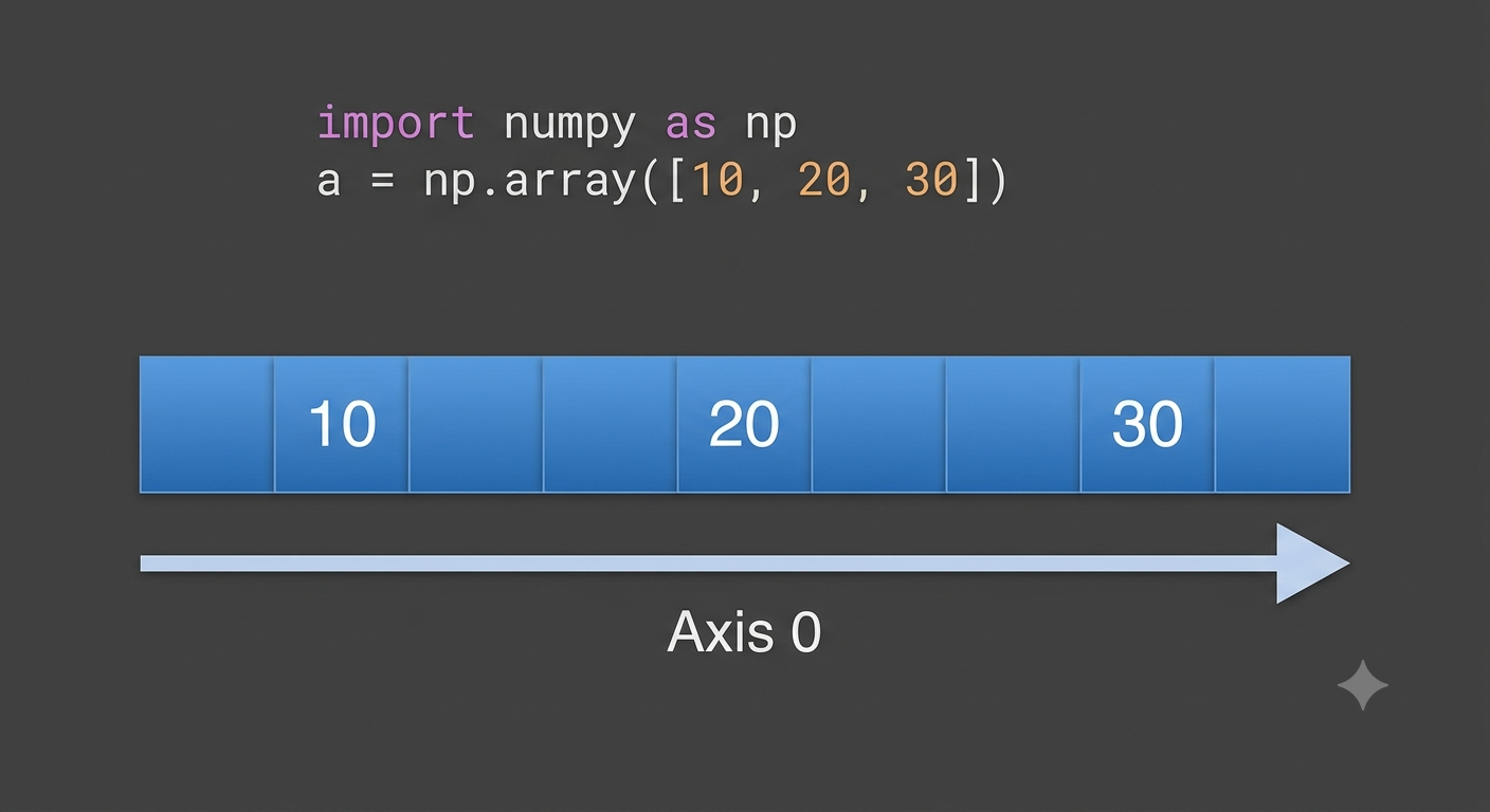
1D Array (The Axis)
We begin with the simplest structure. A 1D array is just a single row of numbers arranged sequentially in memory. We visualize this as a contiguous horizontal line of data blocks.
In NumPy, a direction of movement is called an Axis. This array has only one direction, which is labeled Axis 0.
2D Array (Stacking 1D Arrays)
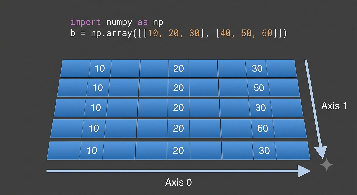
To create a second dimension, we take the original 1D array (the horizontal row [10, 20, 30]) and we stack multiple identical copies of it vertically.
Think of Axis 0 as the columns (the content within each row). The new direction—the stacking direction—is Axis 1 (defining the rows). We now have a physical grid, like a spreadsheet.
3D Array (Stacking 2D Arrays)
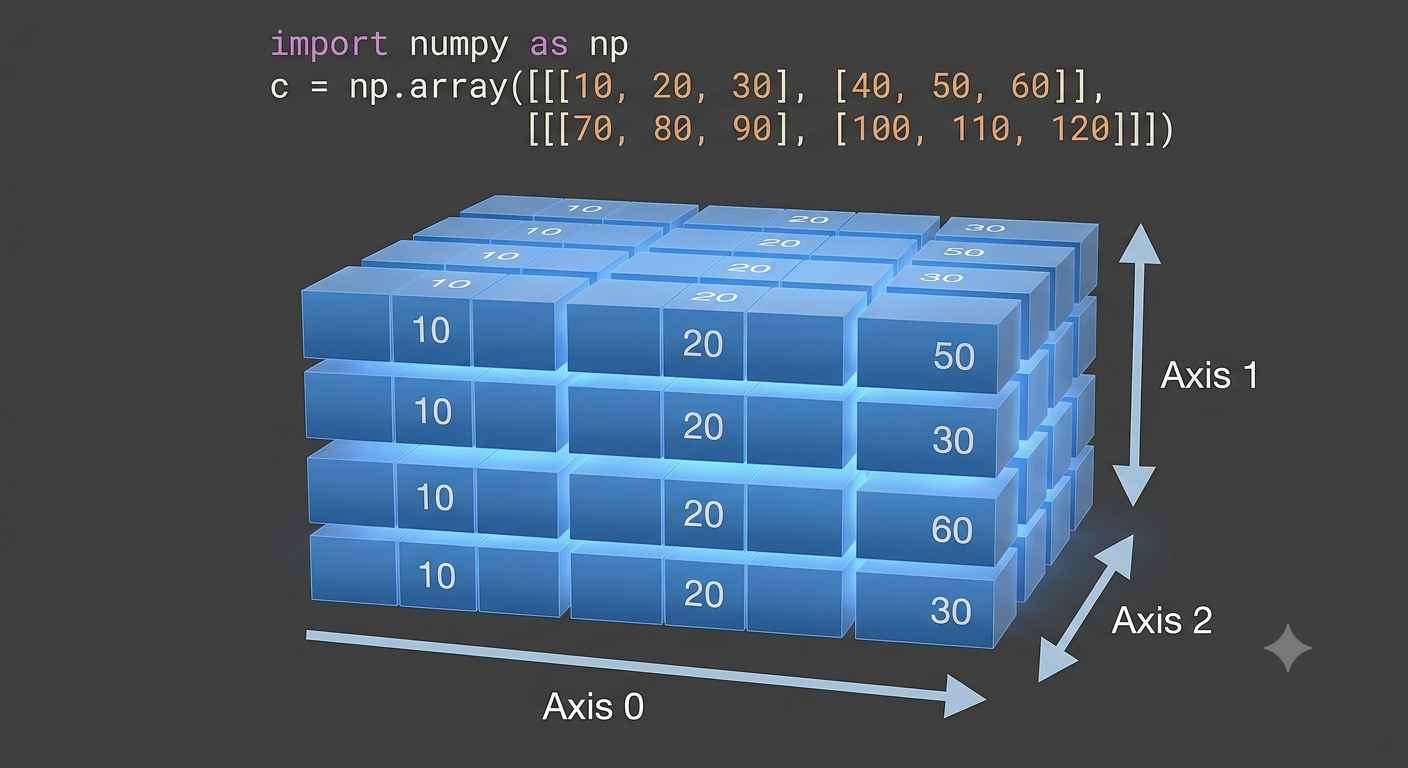
This is a physical volume. To create a 3D volume, we take the entire 2D grid structure from the previous image and we stack multiple copies of it in depth.
We now have three distinct directions of movement: Horizontal (Axis 0), Vertical (Axis 1), and a new stacking direction—Depth—which is labeled Axis 2. This is the structure typically used for simple color images (Height, Width, Channel).
4D Array (Stacking 3D Volumes)
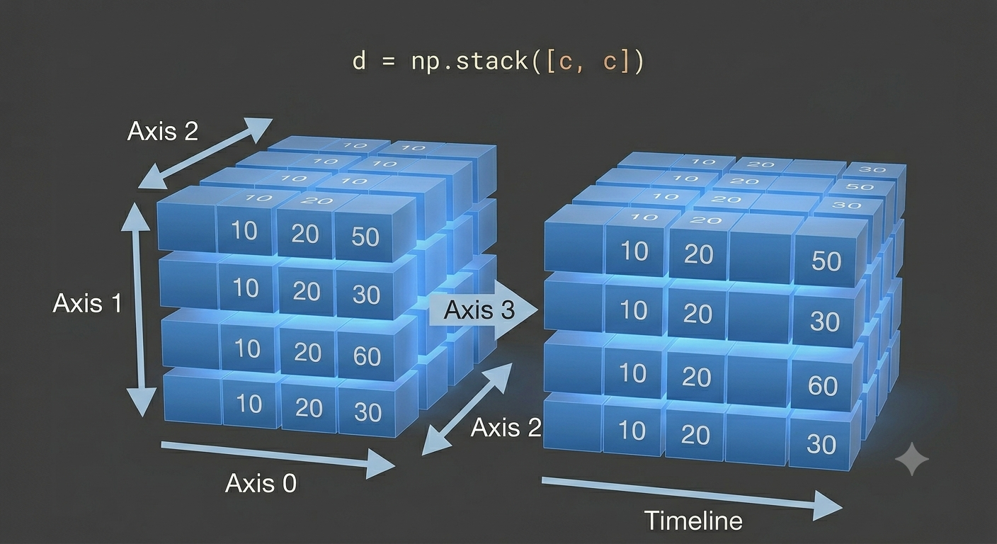
This is where visualization requires a conceptual shift, but the physical mechanic is the same. We treat the entire 3D volume (the complete block from Image 3) as a single, fundamental data unit.
To make 4D, we arrange multiple identical 3D volumes in a sequence, like frames on a filmstrip.
We have now added a new stacking direction—the sequence order—which is labeled Axis 3. This setup is how video data is arranged: a sequence (Axis 3) of volumetric (Height, Width, Channel) images.
Calculating mean along axis
tensor = np.random.rand(4, 5)
tensor
array([[0.63347814, 0.14156362, 0.22217378, 0.17719105, 0.07264797],
       [0.27166672, 0.48655644, 0.45818683, 0.34678748, 0.32654872],
       [0.49915143, 0.19559529, 0.67796101, 0.35525133, 0.71926198],
       [0.12336462, 0.26016002, 0.66256621, 0.90477494, 0.54254784]])
To calculate the mean along the "indexes" we need to consider each row for every column, means we need to calculate it row-wise.
tensor.mean(axis=0)
array([0.38191523, 0.27096884, 0.50522195, 0.4460012 , 0.41525163])
To calculate the mean along the "columns" we need to consider each column for every row, means we need to calculate it column-wise.
tensor.mean(axis=1)
array([0.24941091, 0.37794924, 0.48944421, 0.49868273])