Transform Your Data
Introduction to Transforming Data
Feature engineering is the process of determining which features might be useful in training a model, and then creating those features by transforming raw data found in log files and other sources. In this section, we focus on when and how to transform numeric and categorical data, and the tradeoffs of different approaches.
Reasons for Data Transformation
We transform features primarily for the following reasons:
- Mandatory transformations for data compatibility. Examples include:
- Converting non-numeric features into numeric: You can’t do matrix multiplication on a string, so we must convert the string to some numeric representation.
- Resizing inputs to a fixed size: Linear models and feed-forward neural networks have a fixed number of input nodes, so your input data must always have the same size. For example, image models need to reshape the images in their dataset to a fixed size.
- Optional quality transformations that may help the model perform better. Examples include:
- Tokenization or lower-casing of text features.
- Normalized numeric features (most models perform better afterwards).
- Allowing linear models to introduce non-linearities into the feature space.
Where to Transform?
You can apply transformations either while generating the data on disk, or within the model.
Transforming prior to training
In this approach, we perform the transformation before training. This code lives separate from your machine learning model.
Pros
- Computation is performed only once.
- Computation can look at entire dataset to determine the transformation.
Cons
- Transformations need to be reproduced at prediction time. Beware of skew!
- Any transformation changes require rerunning data generation, leading to slower iterations.
Skew is more dangerous for cases involving online serving. In offline serving, you might be able to reuse the code that generates your training data. In online serving, the code that creates your dataset and the code used to handle live traffic are almost necessarily different, which makes it easy to introduce skew.
Transforming within the model
In this approach, the transformation is part of the model code. The model takes in untransformed data as input and will transform it within the model.
Pros
- Easy iterations.
- If you change the transformations, you can still use the same data files.
- You're guaranteed the same transformations at training and prediction time.
Cons
- Expensive transforms can increase model latency.
- Transformations are per batch.
There are many considerations for transforming per batch. Suppose you want to normalize a feature by its average value—that is, you want to change the feature values to have mean 0 and standard deviation 1. When transforming inside the model, this normalization will have access to only one batch of data, not the full dataset. You can either normalize by the average value within a batch (dangerous if batches are highly variant), or precompute the average and fix it as a constant in the model.
Explore, Clean, and Visualize Your Data
Explore and clean up your data before performing any transformations on it. You may have done some of the following tasks as you collected and constructed your dataset:
- Examine several rows of data.
- Check basic statistics.
- Fix missing numerical entries.
Visualize your data frequently: Graphs can help find anomalies or patterns that aren't clear from numerical statistics. Therefore, before getting too far into analysis, look at your data graphically, either via scatter plots or histograms. View graphs not only at the beginning of the pipeline, but also throughout transformation. Visualizations will help you continually check your assumptions and see the effects of any major changes
Transforming Numeric Data
You may need to apply two kinds of transformations to numeric data:
- Normalizing - transforming numeric data to the same scale as other numeric data.
- Bucketing - transforming numeric (usually continuous) data to categorical data.
Why Normalize Numeric Features?
We strongly recommend normalizing a data set that has numeric features covering distinctly different ranges (for example, age and income). When different features have different ranges, gradient descent can "bounce" and slow down convergence. Optimizers like Adagrad and Adam protect against this problem by creating a separate effective learning rate for each feature.
We also recommend normalizing a single numeric feature that covers a wide range, such as "city population." If you don't normalize the "city population" feature, training the model might generate NaN errors. Unfortunately, optimizers like Adagrad and Adam can't prevent NaN errors when there is a wide range of values within a single feature.
Warning: When normalizing, ensure that the same normalizations are applied at serving time to avoid skew.
Normalization
The goal of normalization is to transform features to be on a similar scale. This improves the performance and training stability of the model.
Four common normalization techniques may be useful:
- scaling to a range
- clipping
- log scaling
- z-score
The following charts show the effect of each normalization technique on the distribution of the raw feature (price) on the left. The charts are based on the data set from 1985 Ward's Automotive Yearbook that is part of the UCI Machine Learning Repository under Automobile Data Set.
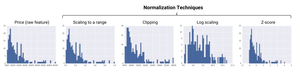 Figure 1. Summary of normalization techniques.
Scaling to a range
Scaling means converting floating-point feature values from their natural range (for example, 100 to 900) into a standard range—usually 0 and 1 (or sometimes -1 to +1). Use the following simple formula to scale to a range:
$$x' = \frac{(x - x_{min})}{(x_{max} - x_{min})}$$
Scaling to a range is a good choice when both of the following conditions are met:
- You know the approximate upper and lower bounds on your data with few or no outliers.
- Your data is approximately uniformly distributed across that range.
A good example is age. Most age values falls between 0 and 90, and every part of the range has a substantial number of people.
In contrast, you would not use scaling on income, because only a few people have very high incomes. The upper bound of the linear scale for income would be very high, and most people would be squeezed into a small part of the scale.
Feature Clipping
Feature clipping caps all feature values above (or below) a certain value to a fixed value if your data set contains extreme outliers. For example, you could clip all temperature values above 40 to be exactly 40.
- You may apply feature clipping before or after other normalizations.
- Formula: Set min/max values to avoid outliers.
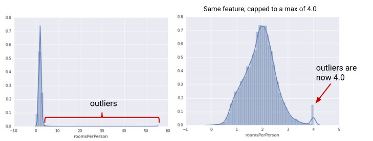 Figure 2. Comparing a raw distribution and its clipped version.
Another simple clipping strategy is to clip by z-score to +-Nσ (for example, limit to +-3σ). Note that σ is the standard deviation.
Log Scaling
Log scaling computes the log of your values to compress a wide range to a narrow range.
$$x' = log(x)$$
- Log scaling is helpful when a handful of your values have many points, while most other values have few points. This data distribution is known as the
power lawdistribution. - Example: Movie ratings are a good example. Most movies have very few ratings (the data in the tail), while a few have lots of ratings (the data in the head).
- Log scaling changes the distribution, helping to improve linear model performance.
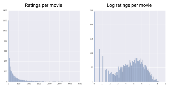 Figure 3. Comparing a raw distribution to its log.
Why log scaling works for skewed data
Log scaling is especially useful for features that span orders of magnitude — for example, money, prices, income, or population. Such features are right-skewed: most values cluster at the low end while a handful are tens or hundreds of times larger. Note that z-score and scaling to a range do not fix skew; they only center and rescale it.
For example, consider home prices:
| Price | log10(price) |
|---|---|
| 300,000 | 5.48 |
| 700,000 | 5.85 |
| 3,000,000 | 6.48 |
| 10,000,000 | 7.00 |
A jump from 3,000,000 to 10,000,000 (a factor of ~3) is only a small step in log space (6.48 → 7.00). This is because log scaling turns multiplicative differences into additive ones: each +1 in log-space means "10× bigger" (for base 10), not "plus 10 dollars". For money, a relative change is usually more meaningful than an absolute one.
Log scaling also makes the skewed distribution look roughly bell-shaped (normal) — the log-normal distribution — which linear models tend to learn more easily.
- Use
log1p(x) = log(1 + x)when your feature can be zero, sincelog(0)is-inf. - Log scaling changes how you interpret coefficients: a weight now measures effect per factor-of-10 increase in the feature, not per +1 unit.
- You must apply the same transformation at inference time to avoid skew.
- Log scaling vs. clipping: clipping compresses the extreme tail of outliers; log scaling compresses the whole range instead. Both prevent a long-tailed feature from hijacking the model — you may even do both.
Z-Score
Z-score is a variation of scaling that represents the number of standard deviations away from the mean.
- You would use z-score to ensure your feature distributions have
mean = 0andstd = 1. - It’s useful when there are a few outliers, but not so extreme that you need clipping.
$$x' = \frac{x - \mu}{\sigma}$$
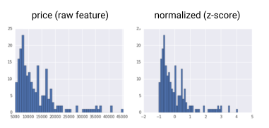 Figure 4. Comparing a raw distribution to its z-score distribution.
Notice that z-score squeezes raw values that have a range of ~40000 down into a range from roughly -1 to +4.
Suppose you're not sure whether the outliers truly are extreme. In this case, start with z-score unless you have feature values that you don't want the model to learn; for example, the values are the result of measurement error or a quirk.
Binning (Bucketing)
Binning (also called bucketing) is a feature engineering technique that groups different numerical subranges into bins or buckets. In many cases, binning turns numerical data into categorical data. For example, consider a feature named X whose lowest value is 15 and highest value is 425. Using binning, you could represent X with the following five bins:
- Bin 1: 15 to 34
- Bin 2: 35 to 117
- Bin 3: 118 to 279
- Bin 4: 280 to 392
- Bin 5: 393 to 425
Bin 1 spans the range 15 to 34, so every value of X between 15 and 34 ends up in Bin 1. A model trained on these bins will react no differently to X values of 17 and 29 since both values are in Bin 1.
The feature vector represents the five bins as follows:
| Bin number | Range | Feature vector |
|---|---|---|
| 1 | 15-34 | [1.0, 0.0, 0.0, 0.0, 0.0] |
| 2 | 35-117 | [0.0, 1.0, 0.0, 0.0, 0.0] |
| 3 | 118-279 | [0.0, 0.0, 1.0, 0.0, 0.0] |
| 4 | 280-392 | [0.0, 0.0, 0.0, 1.0, 0.0] |
| 5 | 393-425 | [0.0, 0.0, 0.0, 0.0, 1.0] |
Even though X is a single column in the dataset, binning causes a model to treat X as five separate features. Therefore, the model learns separate weights for each bin.
Binning is a good alternative to scaling or clipping when either of the following conditions is met:
- The overall linear relationship between the feature and the label is weak or nonexistent.
- When the feature values are clustered.
Binning can feel counterintuitive, given that the model in the previous example treats the values 37 and 115 identically. But when a feature appears more clumpy than linear, binning is a much better way to represent the data.
Binning example: number of shoppers versus temperature
Suppose you are creating a model that predicts the number of shoppers by the outside temperature for that day. Here's a plot of the temperature versus the number of shoppers:
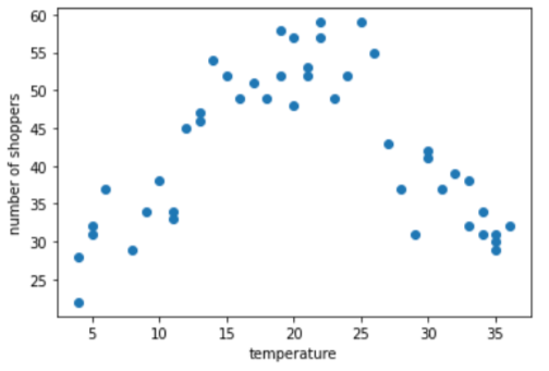
Figure 9. A scatter plot of 45 points.
The plot shows, not surprisingly, that the number of shoppers was highest when the temperature was most comfortable.
You could represent the feature as raw values: a temperature of 35.0 in the dataset would be 35.0 in the feature vector. Is that the best idea?
During training, a linear regression model learns a single weight for each feature. Therefore, if temperature is represented as a single feature, then a temperature of 35.0 would have five times the influence (or one-fifth the influence) in a prediction as a temperature of 7.0. However, the plot doesn't really show any sort of linear relationship between the label and the feature value.
The graph suggests three clusters in the following subranges:
- Bin 1 is the temperature range 4-11.
- Bin 2 is the temperature range 12-26.
- Bin 3 is the temperature range 27-36.
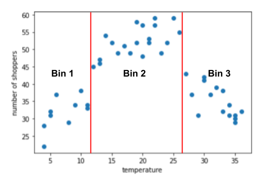
Figure 10. The scatter plot divided into three bins.
The model learns separate weights for each bin.
While it's possible to create more than three bins, even a separate bin for each temperature reading, this is often a bad idea for the following reasons:
- A model can only learn the association between a bin and a label if there are enough examples in that bin. In the given example, each of the 3 bins contains at least 10 examples, which might be sufficient for training. With 33 separate bins, none of the bins would contain enough examples for the model to train on.
- A separate bin for each temperature results in 33 separate temperature features. However, you typically should minimize the number of features in a model.
Quantile Bucketing
Quantile bucketing creates bucketing boundaries such that the number of examples in each bucket is exactly or nearly equal. Quantile bucketing mostly hides the outliers.
To illustrate the problem that quantile bucketing solves, consider the equally spaced buckets shown in the following figure, where each of the ten buckets represents a span of exactly 10,000 dollars. Notice that the bucket from 0 to 10,000 contains dozens of examples but the bucket from 50,000 to 60,000 contains only 5 examples. Consequently, the model has enough examples to train on the 0 to 10,000 bucket but not enough examples to train on for the 50,000 to 60,000 bucket.
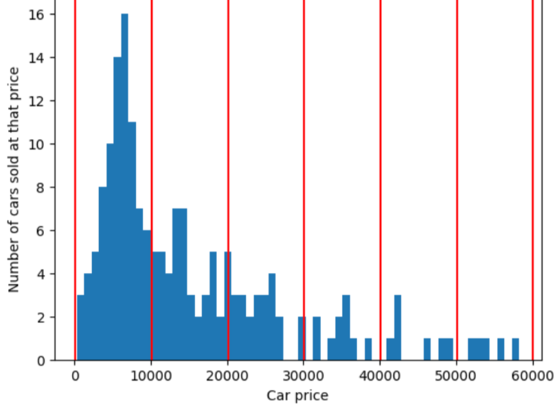
Figure 13. Some buckets contain a lot of cars; other buckets contain very few cars.
In contrast, the following figure uses quantile bucketing to divide car prices into bins with approximately the same number of examples in each bucket. Notice that some of the bins encompass a narrow price span while others encompass a very wide price span.
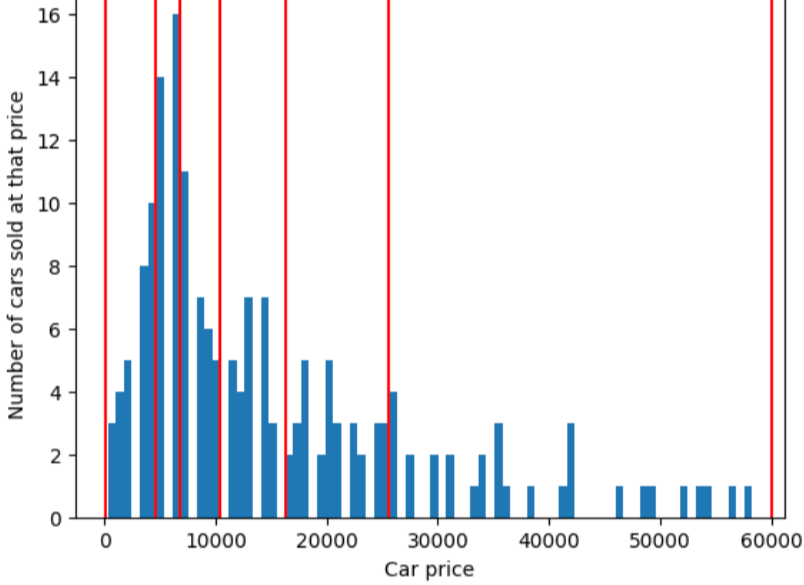
Figure 14. Quantile bucketing gives each bucket about the same number of cars.