Linear Regression
Linear regression is a statistical technique used to find the relationship between variables. In an ML context, linear regression finds the relationship between features and a label.
For example, suppose we want to predict a car's fuel efficiency in miles per gallon based on how heavy the car is, and we have the following dataset:
| Pounds in 1000s (feature) | Miles per gallon (label) |
|---|---|
| 3.5 | 18 |
| 3.69 | 15 |
| 3.44 | 18 |
| 3.43 | 16 |
| 4.34 | 15 |
| 4.42 | 14 |
| 2.37 | 24 |
If we plotted these points, we'd get the following graph:
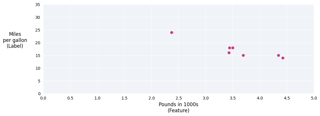 Figure 1. Car heaviness (in pounds) versus miles per gallon rating. As a car gets heavier, its miles per gallon rating generally decreases.
We could create our own model by drawing a best fit line through the points:
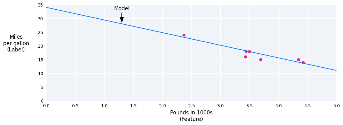 Figure 2. A best fit line drawn through the data from the previous figure.
Equation
In algebraic terms, the model would be defined as $y=mx+c$, where
- $y$ is miles per gallon—the value we want to predict.
- $m$ is the slope of the line.
- $x$ is pounds—our input value.
- $b$ is the y-intercept.
In ML, we write the equation for a linear regression model as follows:
$$y^`=b+w_{1}x_{1}$$
where:
- $y$ is the predicted label—the output.
- $b$ is the bias of the model. Bias is the same concept as the y-intercept in the algebraic equation for a line. In ML, bias is sometimes referred to as $w_{0}$. Bias is a parameter of the model and is calculated during training.
- $w_{1}$ is the weight of the feature. Weight is the same concept as the slope in the algebraic equation for a line. Weight is a parameter of the model and is calculated during training.
- $x_{1}$ is a feature—the input.
During training, the model calculates the weight and bias that produce the best model.
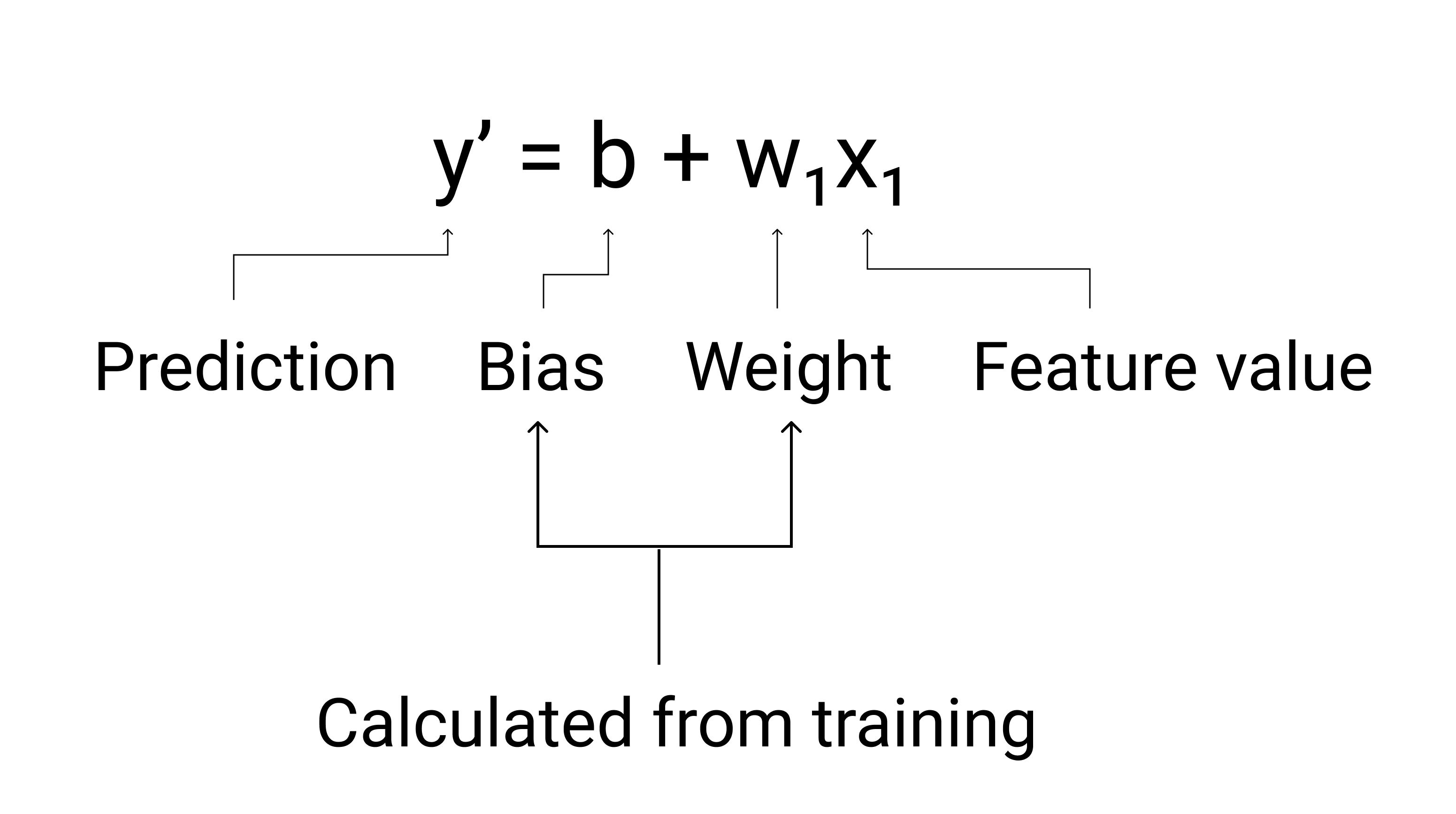 Figure 3. Mathematical representation of a linear model.
In our example, we'd calculate the weight and bias from the line we drew. The bias is 34 (where the line intersects the y-axis), and the weight is –4.6 (the slope of the line). The model would be defined as $y^`=34+(-4.6)(x_{1})$, and we could use it to make predictions. For instance, using this model, a 4,000-pound car would have a predicted fuel efficiency of 15.6 miles per gallon.
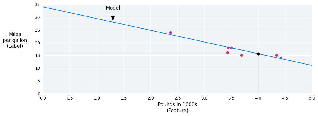 Figure 4. Using the model, a 4,000-pound car has a predicted fuel efficiency of 15.6 miles per gallon.
Models with multiple features
Although the example in this section uses only one feature—the heaviness of the car—a more sophisticated model might rely on multiple features, each having a separate weight ($w_{1}$, $w_{2}$, etc.). For example, a model that relies on five features would be written as follows:
$$y^`=b+w_{1}x_{1}+w_{2}x_{2}+w_{3}x_{3}+w_{4}x_{4}+w_{5}x_{5}$$
For example, a model that predicts gas mileage could additionally use features such as the following:
- Engine displacement
- Acceleration
- Number of cylinders
- Horsepower
This model would be written as follows:
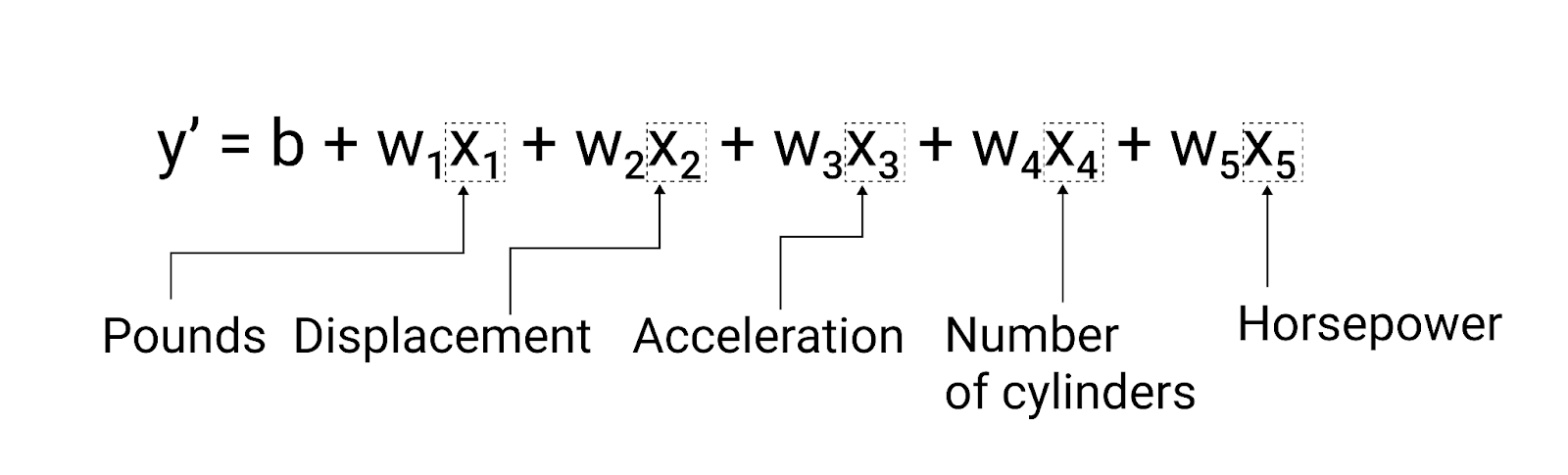 Figure 5. A model with five features to predict a car's miles per gallon rating.
By graphing a couple of these additional features, we can see that they also have a linear relationship to the label, miles per gallon:
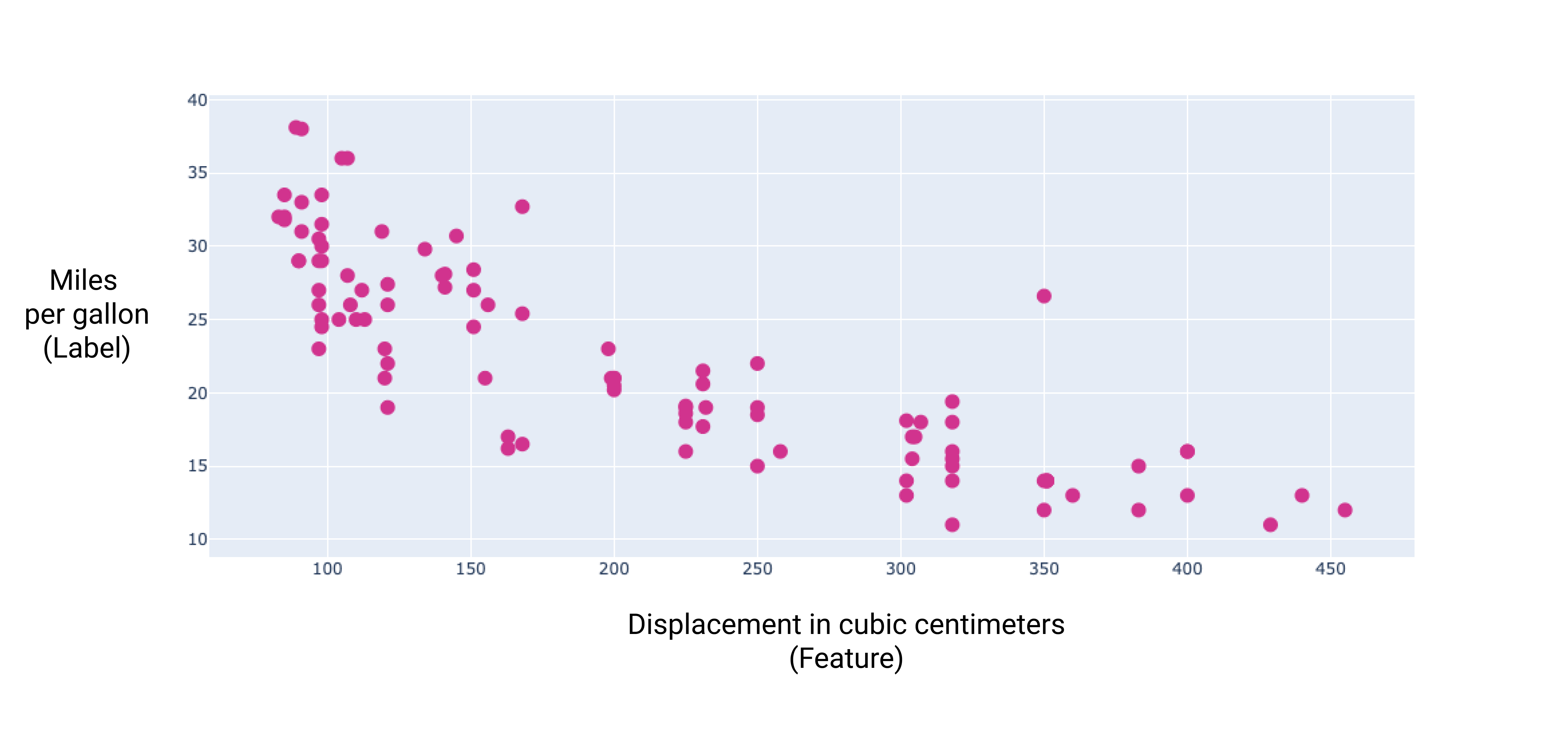 Figure 6. A car's displacement in cubic centimeters and its miles per gallon rating. As a car's engine gets bigger, its miles per gallon rating generally decreases.
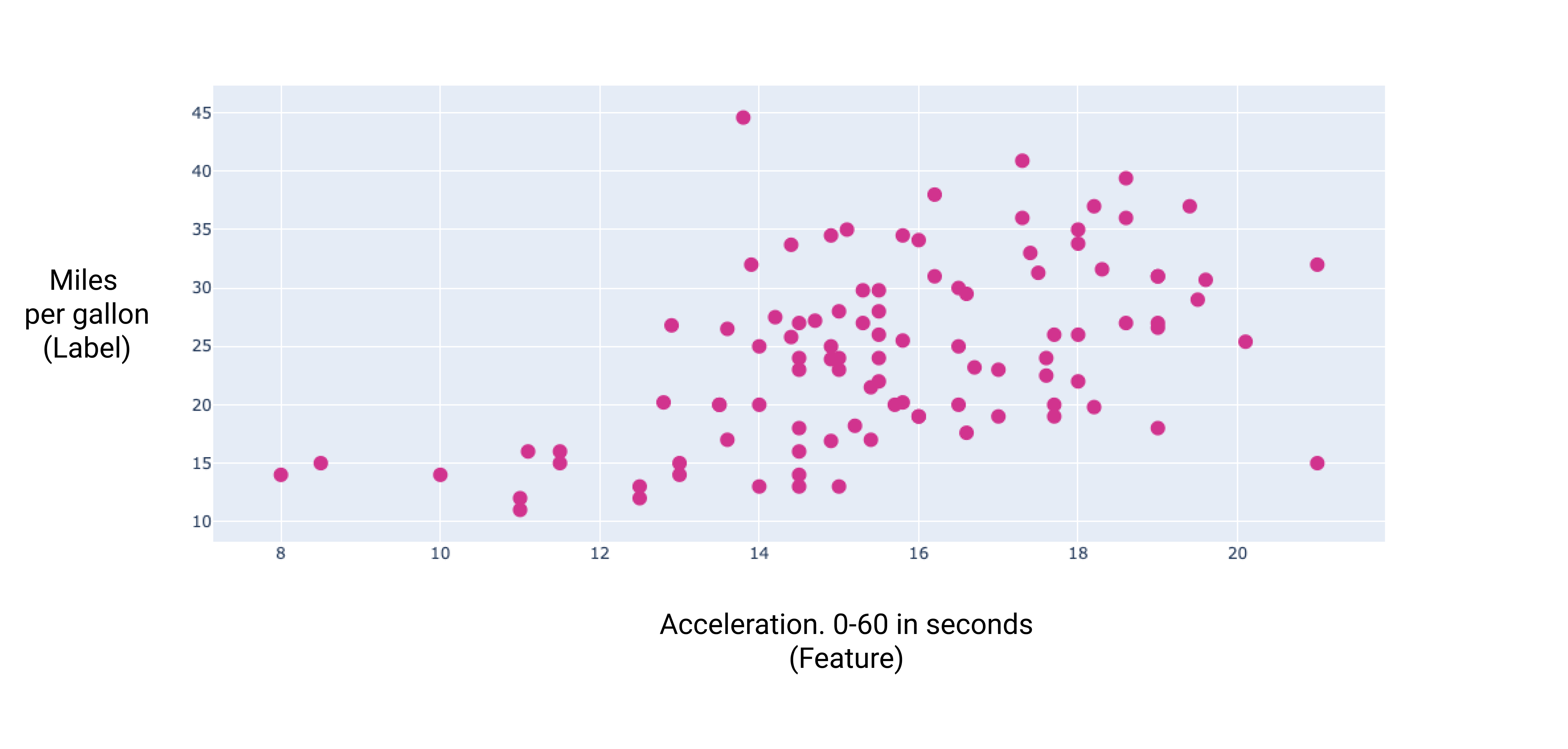 Figure 7. A car's acceleration and its miles per gallon rating. As a car's acceleration takes longer, the miles per gallon rating generally increases.
Loss
Loss is a numerical metric that describes how wrong a model's predictions are. Loss measures the distance between the model's predictions and the actual labels. The goal of training a model is to minimize the loss, reducing it to its lowest possible value.
In the following image, you can visualize loss as arrows drawn from the data points to the model. The arrows show how far the model's predictions are from the actual values.
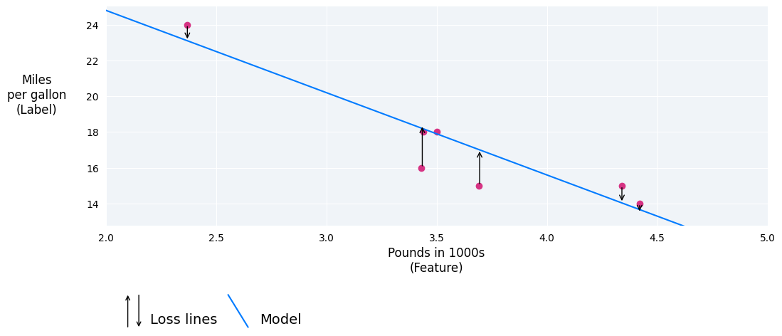 Figure 8. Loss is measured from the actual value to the predicted value.
Distance of loss
In statistics and machine learning, loss measures the difference between the predicted and actual values. Loss focuses on the distance between the values, not the direction. For example, if a model predicts 2, but the actual value is 5, we don't care that the loss is negative (2 – 5= –3). Instead, we care that the distance between the values is 3. Thus, all methods for calculating loss remove the sign.
The two most common methods to remove the sign are the following:
- Take the absolute value of the difference between the actual value and the prediction.
- Square the difference between the actual value and the prediction.
Types of loss
In linear regression, there are five main types of loss, which are outlined in the following table.
| Loss type | Definition | Equation |
|---|---|---|
| $\text{L}_1$ loss | The sum of the absolute values of the difference between the predicted values and the actual values. | $\sum \|\textit{actual value} - \textit{predicted value}\|$ |
| Mean absolute error (MAE) | The average of $\text{L}_1$ losses across a set of $N$ examples. | $\frac{1}{N} \sum \|\textit{actual value} - \textit{predicted value}\|$ |
| $\text{L}_2$ loss | The sum of the squared difference between the predicted values and the actual values. | $\sum (\textit{actual value} - \textit{predicted value})^2$ |
| Mean squared error (MSE) | The average of $\text{L}_2$ losses across a set of $N$ examples. | $\frac{1}{N} \sum (\textit{actual value} - \textit{predicted value})^2$ |
| Root mean squared error (RMSE) | The square root of the mean squared error (MSE). | $\sqrt{\frac{1}{N} \sum (\textit{actual value} - \textit{predicted value})^2}$ |
The functional difference between $L_{1}$ loss and $L_{2}$ loss (or between MAE/RMSE and MSE) is squaring. When the difference between the prediction and label is large, squaring makes the loss even larger. When the difference is small (less than 1), squaring makes the loss even smaller.
Loss metrics like MAE and RMSE may be preferable to $L_{2}$ loss or MSE in some use cases because they tend to be more human-interpretable, as they measure error using the same scale as the model's predicted value.
When processing multiple examples at once, we recommend averaging the losses across all the examples, whether using MAE, MSE, or RMSE.
Calculating loss example
In the previous section, we created the following model to predict fuel efficiency based on car heaviness:
- Model: $y' = 34 + (-4.6)(x_1)$
- Weight: -4.6
- Bias: 34
If the model predicts that a 2,370-pound car gets 23.1 miles per gallon, but it actually gets 24 miles per gallon, we would calculate the $L_2$ loss as follows:
Note: The formula uses 2.37 because the graphs are scaled to 1000s of pounds.
| Value | Equation | Result |
|---|---|---|
| Prediction | $\textit{bias} + (\textit{weight} * \textit{feature value})$ $34 + (-4.6 * 2.37)$ |
23.1 |
| Actual value | $\textit{label}$ | 24 |
| $\text{L}_2$ loss | $(\textit{actual value} - \textit{predicted value})^2$ $(24 - 23.1)^2$ |
0.81 |
In this example, the $\text{L}_2$ loss for that single data point is 0.81.
Choosing a loss
Deciding whether to use MAE or MSE can depend on the dataset and the way you want to handle certain predictions. Most feature values in a dataset typically fall within a distinct range. For example, cars are normally between 2000 and 5000 pounds and get between 8 to 50 miles per gallon. An 8,000-pound car, or a car that gets 100 miles per gallon, is outside the typical range and would be considered an outlier.
An outlier can also refer to how far off a model's predictions are from the real values. For instance, 3,000 pounds is within the typical car-weight range, and 40 miles per gallon is within the typical fuel-efficiency range. However, a 3,000-pound car that gets 40 miles per gallon would be an outlier in terms of the model's prediction because the model would predict that a 3,000-pound car would get around 20 miles per gallon.
When choosing the best loss function, consider how you want the model to treat outliers. For instance, MSE moves the model more toward the outliers, while MAE doesn't. $L_2$ loss incurs a much higher penalty for an outlier than $L_1$ loss. For example, the following images show a model trained using MAE and a model trained using MSE. The red line represents a fully trained model that will be used to make predictions. The outliers are closer to the model trained with MSE than to the model trained with MAE.
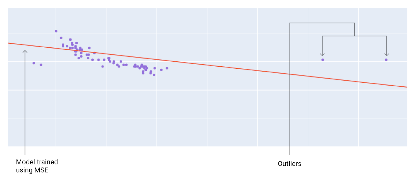 Figure 9. MSE loss moves the model closer to the outliers.
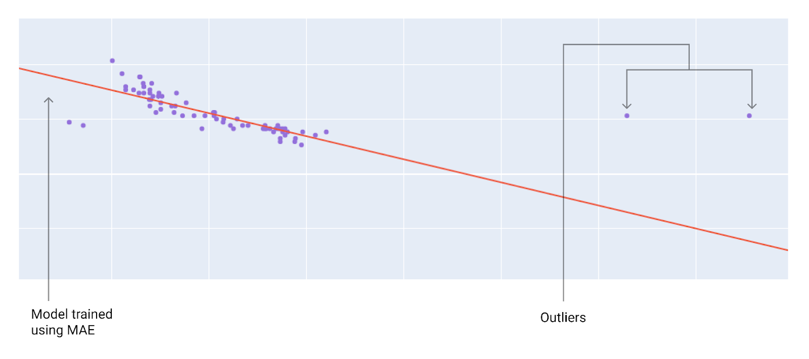 Figure 10. MAE loss keeps the model farther from the outliers.
Note the relationship between the model and the data:
- MSE. The model is closer to the outliers but further away from most of the other data points.
- MAE. The model is further away from the outliers but closer to most of the other data points.
Hyperparameters
Hyperparameters are variables that control different aspects of training. Three common hyperparameters are:
- Learning rate
- Batch size
- Epochs
In contrast, parameters are the variables, like the weights and bias, that are part of the model itself. In other words, hyperparameters are values that you control; parameters are values that the model calculates during training.
Learning rate
Learning rate is a floating point number you set that influences how quickly the model converges. If the learning rate is too low, the model can take a long time to converge. However, if the learning rate is too high, the model never converges, but instead bounces around the weights and bias that minimize the loss. The goal is to pick a learning rate that's not too high nor too low so that the model converges quickly.
The learning rate determines the magnitude of the changes to make to the weights and bias during each step of the gradient descent process. The model multiplies the gradient by the learning rate to determine the model's parameters (weight and bias values) for the next iteration. In the third step of gradient descent, the "small amount" to move in the direction of negative slope refers to the learning rate.
The difference between the old model parameters and the new model parameters is proportional to the slope of the loss function. For example, if the slope is large, the model takes a large step. If small, it takes a small step. For example, if the gradient's magnitude is 2.5 and the learning rate is 0.01, then the model will change the parameter by 0.025.
The ideal learning rate helps the model to converge within a reasonable number of iterations. In Figure 20, the loss curve shows the model significantly improving during the first 20 iterations before beginning to converge:
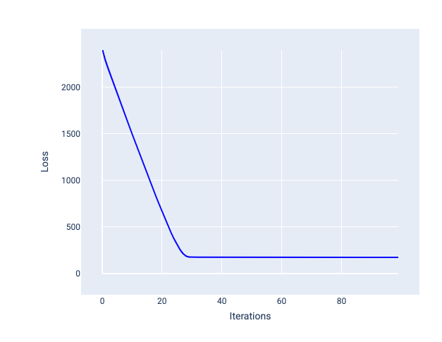
Figure 20. Loss graph showing a model trained with a learning rate that converges quickly.
In contrast, a learning rate that's too small can take too many iterations to converge. In Figure 21, the loss curve shows the model making only minor improvements after each iteration:
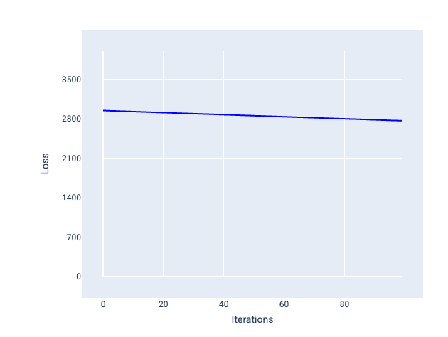
Figure 21. Loss graph showing a model trained with a small learning rate.
A learning rate that's too large never converges because each iteration either causes the loss to bounce around or continually increase. In Figure 22, the loss curve shows the model decreasing and then increasing loss after each iteration, and in Figure 23 the loss increases at later iterations:
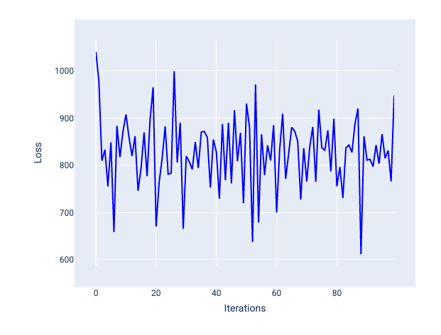
Figure 22. Loss graph showing a model trained with a learning rate that's too big, where the loss curve fluctuates wildly, going up and down as the iterations increase.
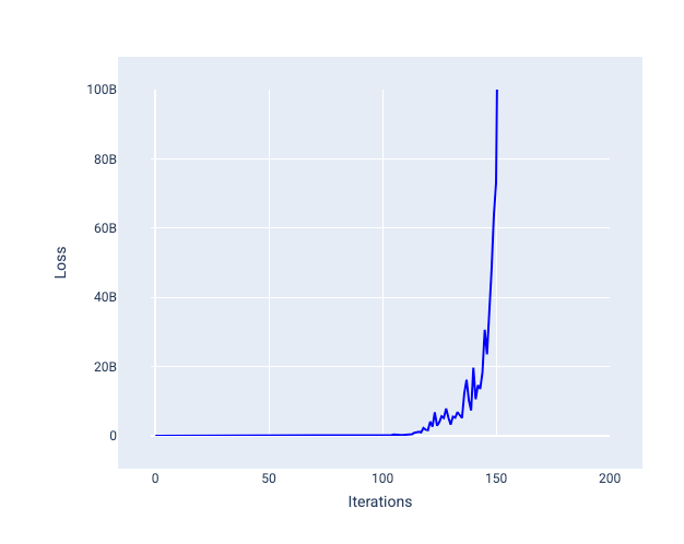
Figure 23. Loss graph showing a model trained with a learning rate that's too big, where the loss curve drastically increases in later iterations.
Batch size
Batch size is a hyperparameter that refers to the number of examples the model processes before updating its weights and bias. You might think that the model should calculate the loss for every example in the dataset before updating the weights and bias. However, when a dataset contains hundreds of thousands or even millions of examples, using the full batch isn't practical.
Two common techniques to get the right gradient on average without needing to look at every example in the dataset before updating the weights and bias are stochastic gradient descent and mini-batch stochastic gradient descent:
- Stochastic gradient descent (SGD): Stochastic gradient descent uses only a single example (a batch size of one) per iteration. Given enough iterations, SGD works but is very noisy. "Noise" refers to variations during training that cause the loss to increase rather than decrease during an iteration. The term "stochastic" indicates that the one example comprising each batch is chosen at random.
Notice in the following image how loss slightly fluctuates as the model updates its weights and bias using SGD, which can lead to noise in the loss graph:
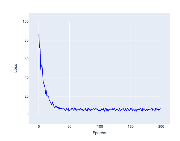
Figure 24. Model trained with stochastic gradient descent (SGD) showing noise in the loss curve.
Note that using stochastic gradient descent can produce noise throughout the entire loss curve, not just near convergence.
- Mini-batch stochastic gradient descent (mini-batch SGD): Mini-batch stochastic gradient descent is a compromise between full-batch and SGD. For N number of data points, the batch size can be any number greater than 1 and less than N. The model chooses the examples included in each batch at random, averages their gradients, and then updates the weights and bias once per iteration.
Determining the number of examples for each batch depends on the dataset and the available compute resources. In general, small batch sizes behaves like SGD, and larger batch sizes behaves like full-batch gradient descent.
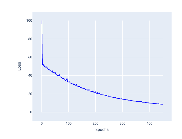
Figure 25. Model trained with mini-batch SGD.
When training a model, you might think that noise is an undesirable characteristic that should be eliminated. However, a certain amount of noise can be a good thing. In later modules, you'll learn how noise can help a model generalize better and find the optimal weights and bias in a neural network.
Epochs
During training, an epoch means that the model has processed every example in the training set once. For example, given a training set with 1,000 examples and a mini-batch size of 100 examples, it will take the model 10 iterations to complete one epoch.
Training typically requires many epochs. That is, the system needs to process every example in the training set multiple times.
The number of epochs is a hyperparameter you set before the model begins training. In many cases, you'll need to experiment with how many epochs it takes for the model to converge. In general, more epochs produces a better model, but also takes more time to train.
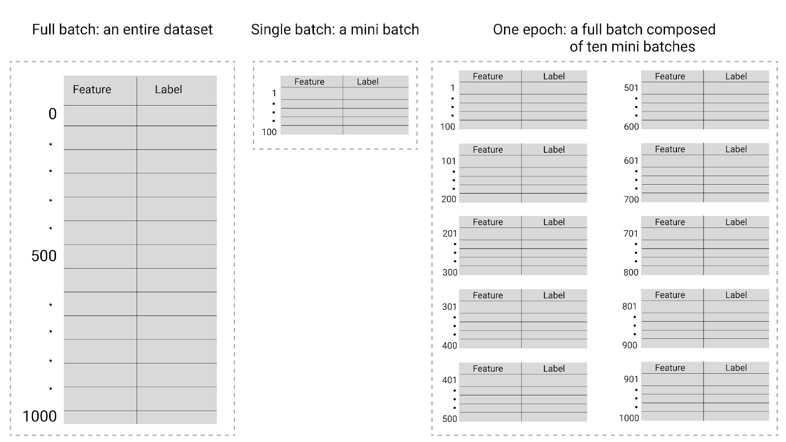
Figure 26. Full batch versus mini batch.
The following table describes how batch size and epochs relate to the number of times a model updates its parameters.
| Batch type | When weights and bias updates occur |
|---|---|
| Full batch | After the model looks at all the examples in the dataset. For instance, if a dataset contains 1,000 examples and the model trains for 20 epochs, the model updates the weights and bias 20 times, once per epoch. |
| Stochastic gradient descent | After the model looks at a single example from the dataset. For instance, if a dataset contains 1,000 examples and trains for 20 epochs, the model updates the weights and bias 20,000 times. |
| Mini-batch stochastic gradient descent | After the model looks at the examples in each batch. For instance, if a dataset contains 1,000 examples, and the batch size is 100, and the model trains for 20 epochs, the model updates the weights and bias 200 times. |